

142
5. Finite Element Methods for Solving Hydrodynamic Dispersion Equations
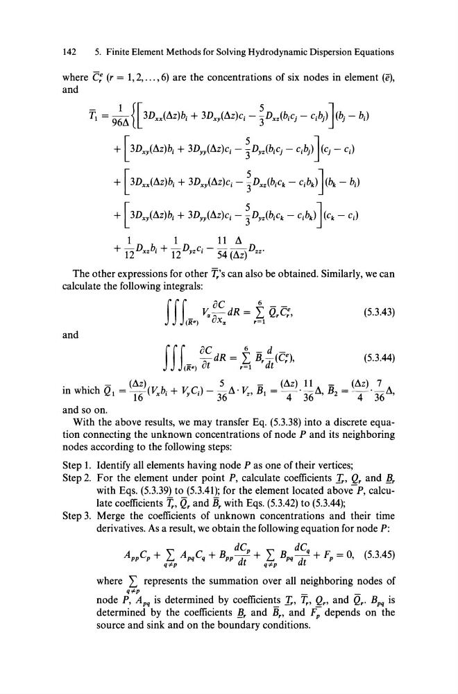
where C: (r = 1,2, ... ,6) are the concentrations of six nodes in element (e),
and
Tl = 9!ß {[3DxAßZ)bi + 3Dx,(ßZ)Ci - ~Dxz(biCj - Cibj)}bj - bi)
+ [3Dxy(ßZ)bi + 3Dyy(ßZ)Ci - ~DyZ
+ [3Dx,(ßZ)bi + 3Dyy(ßZ)Ci - ~Dyz(biCk - Cib,.)}Ck - Ci)
1
1
11 ß
+ 12Dxzbi + 12Dyzci - 54 (ßz)Dzz.
The other expressions for other T,.'s can also be obtained. Similarly, we can
calculate the following integrals:
ffi ac ~ -_ v,.~dR = 1... QrC:,
(Re)
uX,.
r=l
(5.3.43)
and
ffi ac ~ - d -
_ !)dR = 1... Brd-(C:),
(Re) ut
r=l
t
(5.3.44)
.
. -
(Az)
5
-
(ßz) 11
-
(Az) 7
In WhlCh Ql = 16(Vx bj + YyC;) - 36 ß ' v", B1 = 4' 36ß , B2 = 4' 36 ß ,
and so on.
With the above results, we may transfer Eq. (5.3.38) into a discrete equation connecting the unknown concentrations of node P and its neighboring
nodes according to the following steps:
Step 1. Identify all elements having node P as one of their vertices;
Step 2. For the element under point P, calculate coefficients Ir, Qr and llr
with Eqs. (5.3.39) to (5.3.41); for the element located above-P, calculate coefficients T,., Qr and Er with Eqs. (5.3.42) to (5.3.44);
Step 3. Merge the coefficients of unknown concentrations and their time
derivatives. As a result, we obtain the following equation for node P:
"
dC p "
dC q
AppCp + 1... ApqCq + BpP - d + 1... Bpq - d + Fp = 0, (5.3.45)
q,.p
t
q,.p
t
where L represents the summation over all neighboring nodes of
q,.p
node P, Apq is determined by coefficients Ir, T,., Qr' and Qr. Bpq is
determined by the coefficients llr and E" and i; depends on the
source and sink and on the boundary conditions.
5. Finite Element Methods for Solving Hydrodynamic Dispersion Equations
where C: (r = 1,2, ... ,6) are the concentrations of six nodes in element (e),
and
Tl = 9!ß {[3DxAßZ)bi + 3Dx,(ßZ)Ci - ~Dxz(biCj - Cibj)}bj - bi)
+ [3Dxy(ßZ)bi + 3Dyy(ßZ)Ci - ~DyZ
+ [3Dx,(ßZ)bi + 3Dyy(ßZ)Ci - ~Dyz(biCk - Cib,.)}Ck - Ci)
1
1
11 ß
+ 12Dxzbi + 12Dyzci - 54 (ßz)Dzz.
The other expressions for other T,.'s can also be obtained. Similarly, we can
calculate the following integrals:
ffi ac ~ -_ v,.~dR = 1... QrC:,
(Re)
uX,.
r=l
(5.3.43)
and
ffi ac ~ - d -
_ !)dR = 1... Brd-(C:),
(Re) ut
r=l
t
(5.3.44)
.
. -
(Az)
5
-
(ßz) 11
-
(Az) 7
In WhlCh Ql = 16(Vx bj + YyC;) - 36 ß ' v", B1 = 4' 36ß , B2 = 4' 36 ß ,
and so on.
With the above results, we may transfer Eq. (5.3.38) into a discrete equation connecting the unknown concentrations of node P and its neighboring
nodes according to the following steps:
Step 1. Identify all elements having node P as one of their vertices;
Step 2. For the element under point P, calculate coefficients Ir, Qr and llr
with Eqs. (5.3.39) to (5.3.41); for the element located above-P, calculate coefficients T,., Qr and Er with Eqs. (5.3.42) to (5.3.44);
Step 3. Merge the coefficients of unknown concentrations and their time
derivatives. As a result, we obtain the following equation for node P:
"
dC p "
dC q
AppCp + 1... ApqCq + BpP - d + 1... Bpq - d + Fp = 0, (5.3.45)
q,.p
t
q,.p
t
where L represents the summation over all neighboring nodes of
q,.p
node P, Apq is determined by coefficients Ir, T,., Qr' and Qr. Bpq is
determined by the coefficients llr and E" and i; depends on the
source and sink and on the boundary conditions.