

5.3. Finite Element Methods for Three-Dimensional Problems
135
x
- i llz 1 -
z
y
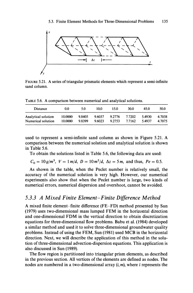
FIGURE 5.21. Aseries oftriangular prismatic elements which represent a semi-infinite
sand column.
TADLE 5.6. A comparison between numerical and analytical solutions.
Distance
0.0
5.0
10.0
15.0
30.0
45.0
50.0
Analytical solution
10.0000
9.8405
9.6037
9.2776
7.7202
5.4930
4.7038
Numerical solution
10.0000
9.8399
9.6023
9.2753
7.7162
5.4937
4.7075
used to represent a semi-infinite sand eolumn as shown in Figure 5.21. A
eomparison between the numerieal solution and analytieal solution is shown
in Table 5.6.
To obtain the solutions listed in Table 5.6, the following data are used:
Co = 10glm 3 , V= Imid, D= 10m 2 1d, L\z=5m, andthus, Pe =0.5.
As shown in the table, when the Peelet number is relatively smalI, the
aeeuraey of the numerieal solution is very high. However, our numerieal
experiments also show that when the Peclet number is large, two kinds of
numerieal errors, numerieal dispersion and overshoot, eannot be avoided.
5.3.3 A Mixed Finite Element-Finite Difference Method
A mixed finite element-finite differenee (FE-FD) method presented by Sun
(1979) uses two-dimensional mass lumped FEM in the horizontal direetion
and one-dimensional FDM in the vertieal direetion to obtain diseretization
equations for three-dimensional flow problems. Babu et al. (1984) developed
a similar method and used it to solve three-dimensional groundwater quality
problems. Instead ofusing the FEM, Sun (1981) used MCB in the horizontal
direetion. Next, we will deseribe the applieation of this method in the solution of three-dimensional adveetion-dispersion equations. This applieation is
also diseussed in Sun (1989).
The flow region is partitioned into triangular prism elements, as deseribed
in the previous seetion. All vertiees of the elements are defined as nodes. The
nodes are numbered in a two-dimensional array (i, m), where i represents the
135
x
- i llz 1 -
z
y
FIGURE 5.21. Aseries oftriangular prismatic elements which represent a semi-infinite
sand column.
TADLE 5.6. A comparison between numerical and analytical solutions.
Distance
0.0
5.0
10.0
15.0
30.0
45.0
50.0
Analytical solution
10.0000
9.8405
9.6037
9.2776
7.7202
5.4930
4.7038
Numerical solution
10.0000
9.8399
9.6023
9.2753
7.7162
5.4937
4.7075
used to represent a semi-infinite sand eolumn as shown in Figure 5.21. A
eomparison between the numerieal solution and analytieal solution is shown
in Table 5.6.
To obtain the solutions listed in Table 5.6, the following data are used:
Co = 10glm 3 , V= Imid, D= 10m 2 1d, L\z=5m, andthus, Pe =0.5.
As shown in the table, when the Peelet number is relatively smalI, the
aeeuraey of the numerieal solution is very high. However, our numerieal
experiments also show that when the Peclet number is large, two kinds of
numerieal errors, numerieal dispersion and overshoot, eannot be avoided.
5.3.3 A Mixed Finite Element-Finite Difference Method
A mixed finite element-finite differenee (FE-FD) method presented by Sun
(1979) uses two-dimensional mass lumped FEM in the horizontal direetion
and one-dimensional FDM in the vertieal direetion to obtain diseretization
equations for three-dimensional flow problems. Babu et al. (1984) developed
a similar method and used it to solve three-dimensional groundwater quality
problems. Instead ofusing the FEM, Sun (1981) used MCB in the horizontal
direetion. Next, we will deseribe the applieation of this method in the solution of three-dimensional adveetion-dispersion equations. This applieation is
also diseussed in Sun (1989).
The flow region is partitioned into triangular prism elements, as deseribed
in the previous seetion. All vertiees of the elements are defined as nodes. The
nodes are numbered in a two-dimensional array (i, m), where i represents the