

5.2. The Multiple Cell Balance Method
115
Step 3. Define basis functions in the local coordinate system. According to
the number and locations of each element, the basis function associated with each node in the local coordinate system can be found
from Tables 5.1 and 5.3 and 5.4.
Step 4. Calculate the Jacobian of co ordinate transformation. Once the basis
functions are determined in the local coordinate system, we will have
the coordinate transformation relation, Eq. (5.1.47), for each element.
Then, we can calculate the Jacobian (5.1.48) and its inverse.
Step 5. Calculate local coefficients Aj~}, B1~}, and Fiel for each element. The
computation should be completed in the local co ordinate system.
When linear or bilinear elements are used, these coefficients are
al ready given explicitly in Section 5.1.2.
Step 6. Calculate global coefficients A i •j , B i • j , and F i These global values can
be obtained by accumulating their local values in all relative elements and incorporating boundary conditions. Thus, the PDE is
transformed into a system of ODE by spatial discretization.
Step 7. Discrete the time domain into time steps. In each time step, the time
derivative in Eq. (5.1.12) is replaced by its finite difference approximation. Thus, the system of ODE in each time step is transformed
into a system of algebraic equations as given in Eq. (5.1.17). The
initial condition is used to determine the right-hand side of this
equation in the first time step.
Step 8. Solve the algebraic system to obtain the concentration distribution
for each time step. This procedure is repeated until the total simulation time is achieved. The right-hand of Eq. (5.1.17) depends on the
solution oflast time step. The solution methods of Eq. (5.1.17) will be
discussed in Seetion 5.4.
5.2 The Multiple Cell Balance Method
5.2.1 Governing Equations
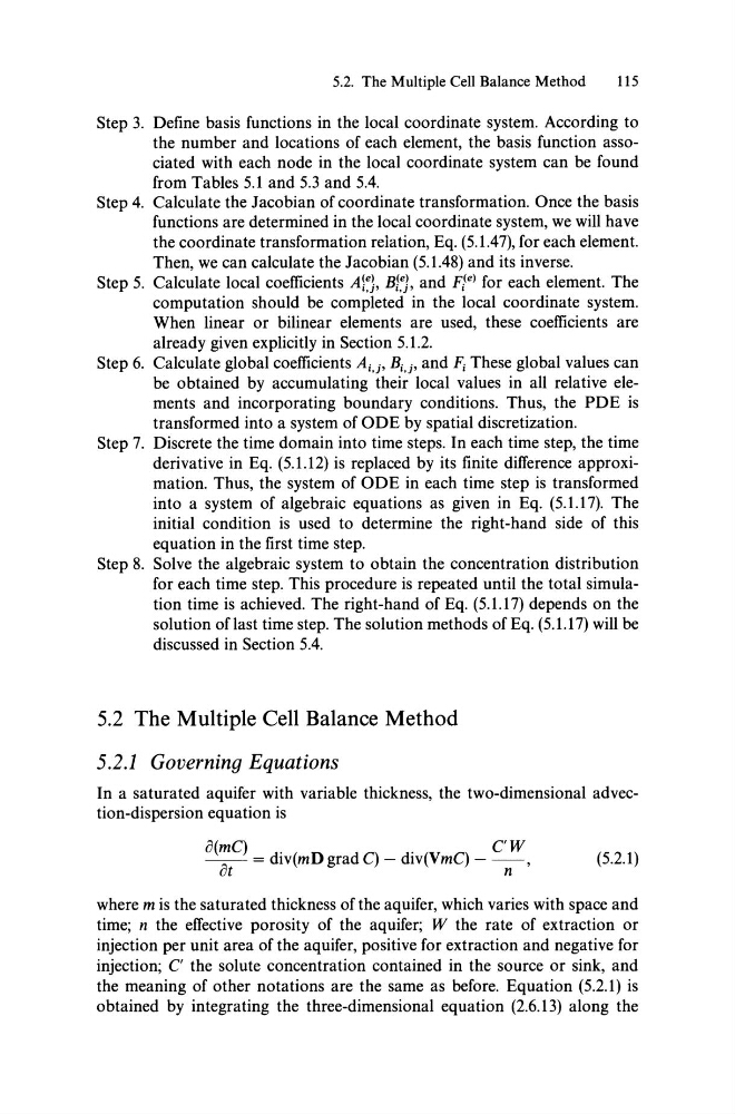
In a saturated aquifer with variable thickness, the two-dimensional advection-dispersion equation is
o(mC) d' (
d) d'
) C' W
-",- = IV mD gra C - IV(VmC - - - ,
ut
n
(5.2.1)
where m is the saturated thickness of the aquifer, which varies with space and
time; n the effective porosity of the aquifer; W the rate of extraction or
injection per unit area of the aquifer, positive for extraction and negative for
injection; C' the solute concentration contained in the source or sink, and
the meaning of other notations are the same as before. Equation (5.2.1) is
obtained by integrating the three-dimensional equation (2.6.13) along the
115
Step 3. Define basis functions in the local coordinate system. According to
the number and locations of each element, the basis function associated with each node in the local coordinate system can be found
from Tables 5.1 and 5.3 and 5.4.
Step 4. Calculate the Jacobian of co ordinate transformation. Once the basis
functions are determined in the local coordinate system, we will have
the coordinate transformation relation, Eq. (5.1.47), for each element.
Then, we can calculate the Jacobian (5.1.48) and its inverse.
Step 5. Calculate local coefficients Aj~}, B1~}, and Fiel for each element. The
computation should be completed in the local co ordinate system.
When linear or bilinear elements are used, these coefficients are
al ready given explicitly in Section 5.1.2.
Step 6. Calculate global coefficients A i •j , B i • j , and F i These global values can
be obtained by accumulating their local values in all relative elements and incorporating boundary conditions. Thus, the PDE is
transformed into a system of ODE by spatial discretization.
Step 7. Discrete the time domain into time steps. In each time step, the time
derivative in Eq. (5.1.12) is replaced by its finite difference approximation. Thus, the system of ODE in each time step is transformed
into a system of algebraic equations as given in Eq. (5.1.17). The
initial condition is used to determine the right-hand side of this
equation in the first time step.
Step 8. Solve the algebraic system to obtain the concentration distribution
for each time step. This procedure is repeated until the total simulation time is achieved. The right-hand of Eq. (5.1.17) depends on the
solution oflast time step. The solution methods of Eq. (5.1.17) will be
discussed in Seetion 5.4.
5.2 The Multiple Cell Balance Method
5.2.1 Governing Equations
In a saturated aquifer with variable thickness, the two-dimensional advection-dispersion equation is
o(mC) d' (
d) d'
) C' W
-",- = IV mD gra C - IV(VmC - - - ,
ut
n
(5.2.1)
where m is the saturated thickness of the aquifer, which varies with space and
time; n the effective porosity of the aquifer; W the rate of extraction or
injection per unit area of the aquifer, positive for extraction and negative for
injection; C' the solute concentration contained in the source or sink, and
the meaning of other notations are the same as before. Equation (5.2.1) is
obtained by integrating the three-dimensional equation (2.6.13) along the