

114
5. Finite Element Methods for Solving Hydrodynamic Dispersion Equations
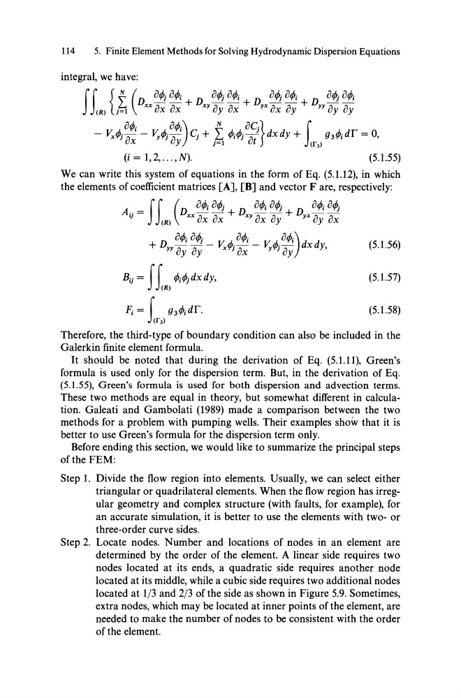
integral, we have:
f r {f (D arA arA + D a,pj a,pi + D a,pj a,pi + D a,pj a,pi
J (R) j=l xx ax ax xy ay ax yx ax ay YY ay ay
a,p.
a,p.)
N
ac.}
i
- Yx,pj-a '- V,A- a ' Cj + ~ ,pi,pj-a J dxdy +
g3,pidr = 0,
x
Y
J=l
t
(r3)
(i = 1,2, ... ,N).
(5.1.55)
We can write this system of equations in the form of Eq. (5.1.12), in which
the elements of coefficient matrices [A], [B] and vector F are, respectively:
A .. = f r (D a,pi a,pj + D a,pi a,pj + D a,pi a,pj
'J
J(R)
xx ax ax
xYax ay
yx ay ax
a,pi a,pj
a,pi
a,pi)
+ Dyy ay ay - Yx,pj ax - Y,.,pj ay dx dy,
(5.1.56)
(5.1.57)
(5.1.58)
Therefore, the third-type of boundary condition can also be included in the
Galerkin finite element formula.
It should be noted that during the derivation of Eq. (5.1.11), Green's
formula is used only for the dispersion term. But, in the derivation of Eq.
(5.1.55), Green's formula is used for both dispersion and advection terms.
These two methods are equal in theory, but somewhat different in calculation. Galeati and Gambolati (1989) made a comparison between the two
methods for a problem with pumping weHs. Their examples show that it is
better to use Green's formula for the dispersion term only.
Before ending this section, we would like to summarize the principal steps
ofthe FEM:
Step 1. Divide the flow region into elements. UsuaHy, we can select either
triangular or quadrilateral elements. When the flow region has irregular geometry and complex structure (with faults, for example), for
an accurate simulation, it is better to use the elements with two- or
three-order curve sides.
Step 2. Locate nodes. Number and locations of nodes in an element are
determined by the order of the element. A linear side requires two
nodes located at its ends, a quadratic side requires another node
located at its middle, while a cubic side requires two additional nodes
located at 1/3 and 2/3 of the side as shown in Figure 5.9. Sometimes,
extra nodes, which may be located at inner points of the element, are
needed to make the number of nodes to be consistent with the order
of the element.
5. Finite Element Methods for Solving Hydrodynamic Dispersion Equations
integral, we have:
f r {f (D arA arA + D a,pj a,pi + D a,pj a,pi + D a,pj a,pi
J (R) j=l xx ax ax xy ay ax yx ax ay YY ay ay
a,p.
a,p.)
N
ac.}
i
- Yx,pj-a '- V,A- a ' Cj + ~ ,pi,pj-a J dxdy +
g3,pidr = 0,
x
Y
J=l
t
(r3)
(i = 1,2, ... ,N).
(5.1.55)
We can write this system of equations in the form of Eq. (5.1.12), in which
the elements of coefficient matrices [A], [B] and vector F are, respectively:
A .. = f r (D a,pi a,pj + D a,pi a,pj + D a,pi a,pj
'J
J(R)
xx ax ax
xYax ay
yx ay ax
a,pi a,pj
a,pi
a,pi)
+ Dyy ay ay - Yx,pj ax - Y,.,pj ay dx dy,
(5.1.56)
(5.1.57)
(5.1.58)
Therefore, the third-type of boundary condition can also be included in the
Galerkin finite element formula.
It should be noted that during the derivation of Eq. (5.1.11), Green's
formula is used only for the dispersion term. But, in the derivation of Eq.
(5.1.55), Green's formula is used for both dispersion and advection terms.
These two methods are equal in theory, but somewhat different in calculation. Galeati and Gambolati (1989) made a comparison between the two
methods for a problem with pumping weHs. Their examples show that it is
better to use Green's formula for the dispersion term only.
Before ending this section, we would like to summarize the principal steps
ofthe FEM:
Step 1. Divide the flow region into elements. UsuaHy, we can select either
triangular or quadrilateral elements. When the flow region has irregular geometry and complex structure (with faults, for example), for
an accurate simulation, it is better to use the elements with two- or
three-order curve sides.
Step 2. Locate nodes. Number and locations of nodes in an element are
determined by the order of the element. A linear side requires two
nodes located at its ends, a quadratic side requires another node
located at its middle, while a cubic side requires two additional nodes
located at 1/3 and 2/3 of the side as shown in Figure 5.9. Sometimes,
extra nodes, which may be located at inner points of the element, are
needed to make the number of nodes to be consistent with the order
of the element.