

112
5. Finite Element Methods for Solving Hydrodynamic Dispersion Equations
TADLE 5.4. Coefficients in Eq. (5.1.46).
Order of side
First order
Second order
Third order
1/2
~~i - (1/2)
(9/8)e - (5/8)
ß.
1/2
""i -(1/ 2)
(9/8),,2 - (5/8)
n nodes altogether in an element (there are seven in the element of Figure 5.9),
then the substitution
{ X = rP1Xl + rP2 X2 + ... + rPnxn'
Y = rP1Yl + rP2Y2 + ... + rPnYn,
(5.1.47)
transforms the element into a standard one in ~'1 coordinates, where (Xi' Yi),
(i = 1,2, ... , n) are the coordinates of node i, and rPi the corresponding basis
function. When we take ~ = ~i' '1 = '1i on the right-hand side of Eq. (5.1.47),
we will have X = Xi' Y = Yi' because the values of basis functions are an zero
except rPi = 1. Thus, the transformation ofEq. (5.1.47) does provide the corresponding relation between points (~i' '1i) and (Xi' y;).
Since the parameters used in coordinate transformation (5.1.47) are identical to those used in determining the unknown concentration in Eq. (5.1.5),
i.e., an of them are basis functions, so this method has the name of isoparametrie finite element method.
After the basis functions and coordinate transformation are determined,
the only problem left is ca1culating the elements of coefficient matrices in Eq.
(5.1.12).
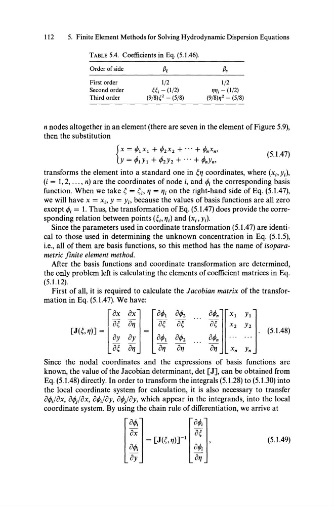
First of an, it is required to calculate the J acobian matrix of the transformation in Eq. (5.1.47). We have:
[
OX OX] [OrPl OrP2 ... orPn] [Xl Yl]
O~ 0'1
O~
O~
O~
X2 Y2
[J(~, '1)] =
=
. (5.1.48)
oy oy
OrPl OrP2
OrPn· . . . ..
-
-
-
-
-
O~ 0'1
0'1 0'1
0'1
Xn Yn
Since the nodal coordinates and the expressions of basis functions are
known, the value of the Jacobian determinant, det [J], can be obtained from
Eq. (5.1.48) direct1y. In order to transform the integrals (5.1.28) to (5.1.30) into
the local coordinate system for ca1culation, it is also necessary to transfer
orPdox, oMox, orPdoy, orPj/oy, which appear in the integrands, into the local
coordinate system. By using the chain rule of differentiation, we arrive at
(5.1.49)
5. Finite Element Methods for Solving Hydrodynamic Dispersion Equations
TADLE 5.4. Coefficients in Eq. (5.1.46).
Order of side
First order
Second order
Third order
1/2
~~i - (1/2)
(9/8)e - (5/8)
ß.
1/2
""i -(1/ 2)
(9/8),,2 - (5/8)
n nodes altogether in an element (there are seven in the element of Figure 5.9),
then the substitution
{ X = rP1Xl + rP2 X2 + ... + rPnxn'
Y = rP1Yl + rP2Y2 + ... + rPnYn,
(5.1.47)
transforms the element into a standard one in ~'1 coordinates, where (Xi' Yi),
(i = 1,2, ... , n) are the coordinates of node i, and rPi the corresponding basis
function. When we take ~ = ~i' '1 = '1i on the right-hand side of Eq. (5.1.47),
we will have X = Xi' Y = Yi' because the values of basis functions are an zero
except rPi = 1. Thus, the transformation ofEq. (5.1.47) does provide the corresponding relation between points (~i' '1i) and (Xi' y;).
Since the parameters used in coordinate transformation (5.1.47) are identical to those used in determining the unknown concentration in Eq. (5.1.5),
i.e., an of them are basis functions, so this method has the name of isoparametrie finite element method.
After the basis functions and coordinate transformation are determined,
the only problem left is ca1culating the elements of coefficient matrices in Eq.
(5.1.12).
First of an, it is required to calculate the J acobian matrix of the transformation in Eq. (5.1.47). We have:
[
OX OX] [OrPl OrP2 ... orPn] [Xl Yl]
O~ 0'1
O~
O~
O~
X2 Y2
[J(~, '1)] =
=
. (5.1.48)
oy oy
OrPl OrP2
OrPn· . . . ..
-
-
-
-
-
O~ 0'1
0'1 0'1
0'1
Xn Yn
Since the nodal coordinates and the expressions of basis functions are
known, the value of the Jacobian determinant, det [J], can be obtained from
Eq. (5.1.48) direct1y. In order to transform the integrals (5.1.28) to (5.1.30) into
the local coordinate system for ca1culation, it is also necessary to transfer
orPdox, oMox, orPdoy, orPj/oy, which appear in the integrands, into the local
coordinate system. By using the chain rule of differentiation, we arrive at
(5.1.49)