

74
M. Fingas
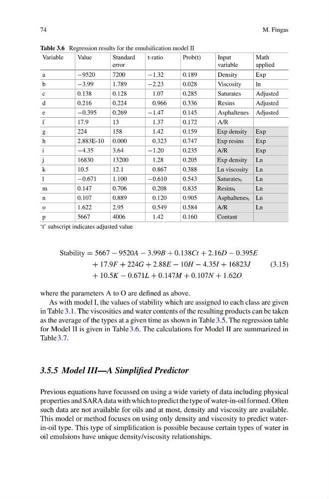
Table 3.6 Regression results for the emulsification model II
Variable
Value
Standard
error
t-ratio
Prob(t)
Input
variable
Math
applied
a
−9520
7200
−1.32
0.189
Density
Exp
b
−3.99
1.789
−2.23
0.028
Viscosity
ln
c
0.138
0.128
1.07
0.285
Saturates
Adjusted
d
0.216
0.224
0.966
0.336
Resins
Adjusted
e
−0.395
0.269
−1.47
0.145
Asphaltenes Adjusted
f
17.9
13
1.37
0.172
A/R
g
224
158
1.42
0.159
Exp density Exp
h
2.883E-10 0.000
0.323
0.747
Exp resins
Exp
i
−4.35
3.64
−1.20
0.235
A/R
Exp
j
16830
13200
1.28
0.205
Exp density Ln
k
10.5
12.1
0.867
0.388
Ln viscosity Ln
l
−0.671
1.100
−0.610
0.543
Saturates t
Ln
m
0.147
0.706
0.208
0.835
Resins t
Ln
n
0.107
0.889
0.120
0.905
Asphaltenes t Ln
o
1.622
2.95
0.549
0.584
A/R
Ln
p
5667
4006
1.42
0.160
Contant
‘t’ subscript indicates adjusted value
Stability = 5667 − 9520A − 3.99B + 0.138Ct + 2.16D − 0.395E
+ 17.9F + 224G + 2.88E − 10H − 4.35I + 16823J
(3.15)
+ 10.5K − 0.671L + 0.147M + 0.107N + 1.62O
where the parameters A to O are defined as above.
As with model I, the values of stability which are assigned to each class are given
in Table 3.1. The viscosities and water contents of the resulting products can be taken
as the average of the types at a given time as shown in Table 3.5. The regression table
for Model II is given in Table 3.6. The calculations for Model II are summarized in
Table 3.7.
3.5.5 Model III—A Simplified Predictor
Previous equations have focussed on using a wide variety of data including physical
properties and SARA data with which to predict the type of water-in-oil formed. Often
such data are not available for oils and at most, density and viscosity are available.
This model or method focuses on using only density and viscosity to predict waterin-oil type. This type of simplification is possible because certain types of water in
oil emulsions have unique density/viscosity relationships.
M. Fingas
Table 3.6 Regression results for the emulsification model II
Variable
Value
Standard
error
t-ratio
Prob(t)
Input
variable
Math
applied
a
−9520
7200
−1.32
0.189
Density
Exp
b
−3.99
1.789
−2.23
0.028
Viscosity
ln
c
0.138
0.128
1.07
0.285
Saturates
Adjusted
d
0.216
0.224
0.966
0.336
Resins
Adjusted
e
−0.395
0.269
−1.47
0.145
Asphaltenes Adjusted
f
17.9
13
1.37
0.172
A/R
g
224
158
1.42
0.159
Exp density Exp
h
2.883E-10 0.000
0.323
0.747
Exp resins
Exp
i
−4.35
3.64
−1.20
0.235
A/R
Exp
j
16830
13200
1.28
0.205
Exp density Ln
k
10.5
12.1
0.867
0.388
Ln viscosity Ln
l
−0.671
1.100
−0.610
0.543
Saturates t
Ln
m
0.147
0.706
0.208
0.835
Resins t
Ln
n
0.107
0.889
0.120
0.905
Asphaltenes t Ln
o
1.622
2.95
0.549
0.584
A/R
Ln
p
5667
4006
1.42
0.160
Contant
‘t’ subscript indicates adjusted value
Stability = 5667 − 9520A − 3.99B + 0.138Ct + 2.16D − 0.395E
+ 17.9F + 224G + 2.88E − 10H − 4.35I + 16823J
(3.15)
+ 10.5K − 0.671L + 0.147M + 0.107N + 1.62O
where the parameters A to O are defined as above.
As with model I, the values of stability which are assigned to each class are given
in Table 3.1. The viscosities and water contents of the resulting products can be taken
as the average of the types at a given time as shown in Table 3.5. The regression table
for Model II is given in Table 3.6. The calculations for Model II are summarized in
Table 3.7.
3.5.5 Model III—A Simplified Predictor
Previous equations have focussed on using a wide variety of data including physical
properties and SARA data with which to predict the type of water-in-oil formed. Often
such data are not available for oils and at most, density and viscosity are available.
This model or method focuses on using only density and viscosity to predict waterin-oil type. This type of simplification is possible because certain types of water in
oil emulsions have unique density/viscosity relationships.