

2 A Strategy for Bioremediation of Marine Shorelines …
33
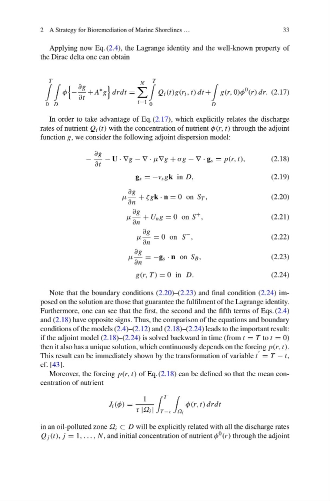
Applying now Eq. (2.4), the Lagrange identity and the well-known property of
the Dirac delta one can obtain
T
0
D
φ
−
∂g
∂t
+ A
∗ g
drdt =
N
i=1
T
0
Q i (t)g(r i , t) dt +
D
g(r, 0)φ
0
(r ) dr. (2.17)
In order to take advantage of Eq. (2.17), which explicitly relates the discharge
rates of nutrient Q i (t) with the concentration of nutrient φ(r, t) through the adjoint
function g, we consider the following adjoint dispersion model:
−
∂g
∂t
− U · ∇g − ∇ · μ∇g + σ g − ∇ · g s = p(r, t),
(2.18)
g s = −v s gk in D,
(2.19)
μ
∂g
∂n
+ ζ gk · n = 0 on S T ,
(2.20)
μ
∂g
∂n
+ U n g = 0 on S
+
,
(2.21)
μ
∂g
∂n
= 0 on S
−
,
(2.22)
μ
∂g
∂n
= −g s · n on S B ,
(2.23)
g(r, T ) = 0 in D.
(2.24)
Note that the boundary conditions (2.20)–(2.23) and final condition (2.24) imposed on the solution are those that guarantee the fulfilment of the Lagrange identity.
Furthermore, one can see that the first, the second and the fifth terms of Eqs. (2.4)
and (2.18) have opposite signs. Thus, the comparison of the equations and boundary
conditions of the models (2.4)–(2.12) and (2.18)–(2.24) leads to the important result:
if the adjoint model (2.18)–(2.24) is solved backward in time (from t = T to t = 0)
then it also has a unique solution, which continuously depends on the forcing p(r, t).
This result can be immediately shown by the transformation of variable t
= T − t,
cf. [43].
Moreover, the forcing p(r, t) of Eq. (2.18) can be defined so that the mean concentration of nutrient
J i (φ) =
1
τ |Ω i |
T
T −τ
Ω i
φ(r, t) drdt
in an oil-polluted zone Ω i ⊂ D will be explicitly related with all the discharge rates
Q j (t), j = 1, . . . , N , and initial concentration of nutrient φ 0 (r ) through the adjoint
33
Applying now Eq. (2.4), the Lagrange identity and the well-known property of
the Dirac delta one can obtain
T
0
D
φ
−
∂g
∂t
+ A
∗ g
drdt =
N
i=1
T
0
Q i (t)g(r i , t) dt +
D
g(r, 0)φ
0
(r ) dr. (2.17)
In order to take advantage of Eq. (2.17), which explicitly relates the discharge
rates of nutrient Q i (t) with the concentration of nutrient φ(r, t) through the adjoint
function g, we consider the following adjoint dispersion model:
−
∂g
∂t
− U · ∇g − ∇ · μ∇g + σ g − ∇ · g s = p(r, t),
(2.18)
g s = −v s gk in D,
(2.19)
μ
∂g
∂n
+ ζ gk · n = 0 on S T ,
(2.20)
μ
∂g
∂n
+ U n g = 0 on S
+
,
(2.21)
μ
∂g
∂n
= 0 on S
−
,
(2.22)
μ
∂g
∂n
= −g s · n on S B ,
(2.23)
g(r, T ) = 0 in D.
(2.24)
Note that the boundary conditions (2.20)–(2.23) and final condition (2.24) imposed on the solution are those that guarantee the fulfilment of the Lagrange identity.
Furthermore, one can see that the first, the second and the fifth terms of Eqs. (2.4)
and (2.18) have opposite signs. Thus, the comparison of the equations and boundary
conditions of the models (2.4)–(2.12) and (2.18)–(2.24) leads to the important result:
if the adjoint model (2.18)–(2.24) is solved backward in time (from t = T to t = 0)
then it also has a unique solution, which continuously depends on the forcing p(r, t).
This result can be immediately shown by the transformation of variable t
= T − t,
cf. [43].
Moreover, the forcing p(r, t) of Eq. (2.18) can be defined so that the mean concentration of nutrient
J i (φ) =
1
τ |Ω i |
T
T −τ
Ω i
φ(r, t) drdt
in an oil-polluted zone Ω i ⊂ D will be explicitly related with all the discharge rates
Q j (t), j = 1, . . . , N , and initial concentration of nutrient φ 0 (r ) through the adjoint