

49
reflecting in a quite natural way the effect of stratification. On the other hand, the influence of
M2 on S and S is completely counterintuitive. Indeed, increasing M2 leads to a decrease of S
u
c
u
and S c' which may not be appropriate.
Imagine that, for some reason, M2 is increasing at a given location in the domain of interest.
This would lead to a decrease of K u ' which might allow a further increase of the shear, since
the turbulent stress, Kudu/dz, is unlikely to exhibit wild variations. Indeed, the order of
magnitude of KuM is commonly thought to be prescribed by the stress driving the turbulent
boundary layer, i.e., the surface wind stress or the bottom stress. Thus, a positive feedback
may develop, possibly leading to a "discontinuity in the velocity" (Mellor and Yamada, 1982),
which would obviously be an artefact. In other words, the velocity field may possibly present
unphysical oscillations in the vertical direction.
To prevent regions of exceedingly high shear from developing, a limitation of Ai2 has been
considered (Mellor and Yamada, 1982), as well as a numerical filtering procedure of ~f2
(Mellor, personal communication). Instead of trying to constrain, in a rather artificial way, the
evolution of some variables of the turbulence model, it may seem desirable to improve the
model by reappraising some of the assumptions underlying its parameterizations. This was
achieved by Galperin et al. (1988), who devised the so-called quasi-equilibrium version of the
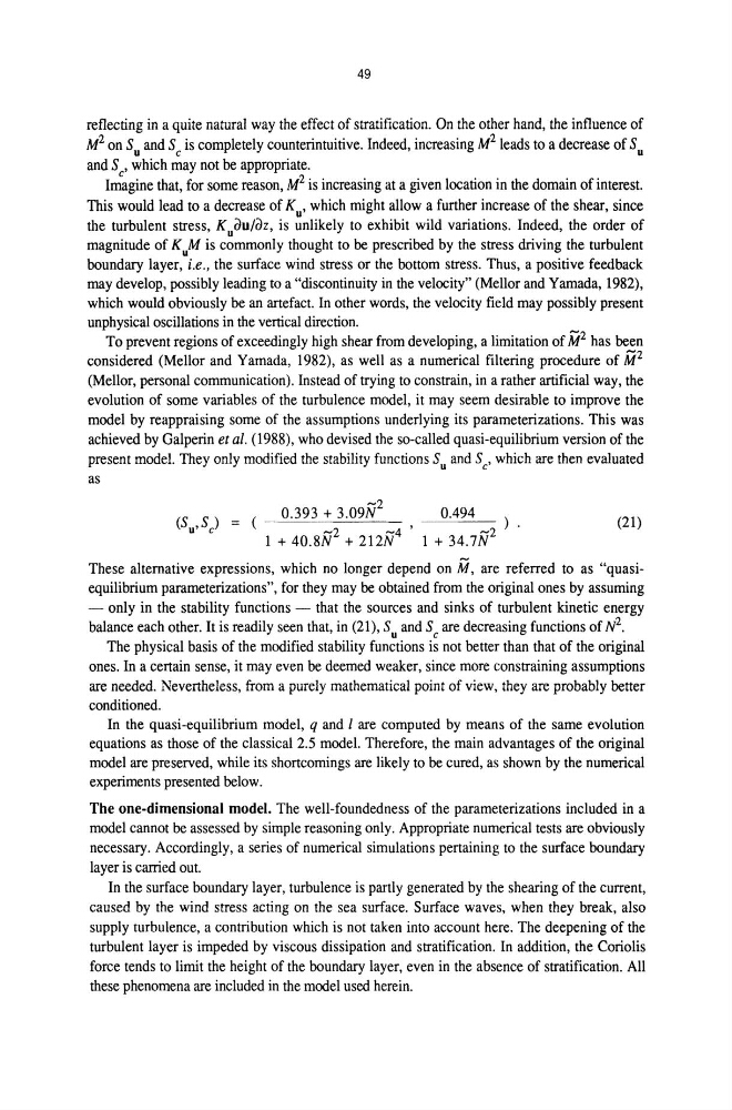
present model. They only modified the stability functions S u and S c' which are then evaluated
as
-2
( s S) = ( 0.393 + 3.09N
0.494) .
u' c
2
4 •
2
1 + 40.8N + 212N
1 + 34.7N
(21)
These alternative expressions, which no longer depend on M, are referred to as "quasiequilibrium parameterizations", for they may be obtained from the original ones by assuming
- only in the stability functions - that the sources and sinks of turbulent kinetic energy
balance each other. It is readily seen that, in (21), Su and Scare decreasing functions of N 2 .
The physical basis of the modified stability functions is not better than that of the original
ones. In a certain sense, it may even be deemed weaker, since more constraining assumptions
are needed. Nevertheless, from a purely mathematical point of view, they are probably better
conditioned.
In the quasi-equilibrium model, q and 1 are computed by means of the same evolution
equations as those of the classical 2.5 model. Therefore, the main advantages of the original
model are preserved, while its shortcomings are likely to be cured, as shown by the numerical
experiments presented below.
The one-dimensional model. The well-foundedness of the parameterizations included in a
model cannot be assessed by simple reasoning only. Appropriate numerical tests are obviously
necessary. Accordingly, a series of numerical simulations pertaining to the surface boundary
layer is carried out.
In the surface boundary layer, turbulence is partly generated by the shearing of the current,
caused by the wind stress acting on the sea surface. Surface waves, when they break, also
supply turbulence, a contribution which is not taken into account here. The deepening of the
turbulent layer is impeded by viscous dissipation and stratification. In addition, the Coriolis
force tends to limit the height of the boundary layer, even in the absence of stratification. All
these phenomena are included in the model used herein.
reflecting in a quite natural way the effect of stratification. On the other hand, the influence of
M2 on S and S is completely counterintuitive. Indeed, increasing M2 leads to a decrease of S
u
c
u
and S c' which may not be appropriate.
Imagine that, for some reason, M2 is increasing at a given location in the domain of interest.
This would lead to a decrease of K u ' which might allow a further increase of the shear, since
the turbulent stress, Kudu/dz, is unlikely to exhibit wild variations. Indeed, the order of
magnitude of KuM is commonly thought to be prescribed by the stress driving the turbulent
boundary layer, i.e., the surface wind stress or the bottom stress. Thus, a positive feedback
may develop, possibly leading to a "discontinuity in the velocity" (Mellor and Yamada, 1982),
which would obviously be an artefact. In other words, the velocity field may possibly present
unphysical oscillations in the vertical direction.
To prevent regions of exceedingly high shear from developing, a limitation of Ai2 has been
considered (Mellor and Yamada, 1982), as well as a numerical filtering procedure of ~f2
(Mellor, personal communication). Instead of trying to constrain, in a rather artificial way, the
evolution of some variables of the turbulence model, it may seem desirable to improve the
model by reappraising some of the assumptions underlying its parameterizations. This was
achieved by Galperin et al. (1988), who devised the so-called quasi-equilibrium version of the
present model. They only modified the stability functions S u and S c' which are then evaluated
as
-2
( s S) = ( 0.393 + 3.09N
0.494) .
u' c
2
4 •
2
1 + 40.8N + 212N
1 + 34.7N
(21)
These alternative expressions, which no longer depend on M, are referred to as "quasiequilibrium parameterizations", for they may be obtained from the original ones by assuming
- only in the stability functions - that the sources and sinks of turbulent kinetic energy
balance each other. It is readily seen that, in (21), Su and Scare decreasing functions of N 2 .
The physical basis of the modified stability functions is not better than that of the original
ones. In a certain sense, it may even be deemed weaker, since more constraining assumptions
are needed. Nevertheless, from a purely mathematical point of view, they are probably better
conditioned.
In the quasi-equilibrium model, q and 1 are computed by means of the same evolution
equations as those of the classical 2.5 model. Therefore, the main advantages of the original
model are preserved, while its shortcomings are likely to be cured, as shown by the numerical
experiments presented below.
The one-dimensional model. The well-foundedness of the parameterizations included in a
model cannot be assessed by simple reasoning only. Appropriate numerical tests are obviously
necessary. Accordingly, a series of numerical simulations pertaining to the surface boundary
layer is carried out.
In the surface boundary layer, turbulence is partly generated by the shearing of the current,
caused by the wind stress acting on the sea surface. Surface waves, when they break, also
supply turbulence, a contribution which is not taken into account here. The deepening of the
turbulent layer is impeded by viscous dissipation and stratification. In addition, the Coriolis
force tends to limit the height of the boundary layer, even in the absence of stratification. All
these phenomena are included in the model used herein.