

41
at the North Pole, with standard spherical coordinates. To avoid dealing with three-dimensional
velocity fields, the results are analysed with the help of the so-called meridional stream function
technique.
Before examining the specific problems listed above, the equations of marine
hydrodynamics are briefly established (Section 2).
2. Equations of marine hydrodynamics
The equations governing marine hydrodynamics processes are derived from the general
theory of fluid mechanics.
Reynolds (1883) realized that there are two types of fluid flow, the laminar mode and the
turbulent mode, in which apparently erratic fluctuations occur. Reynolds (1894) suggested
filtering out the fluctuations and concentrating on the "mean" flow, considered as a laminar one
with modified properties and equations.
Reynolds mostly studied flows he could produce in his laboratory, i.e., small-scale flows.
In the ocean, however, analogous turbulent processes may be found in the surface and bottom
boundary layers, the thickness of which is of order 10-100 m for the former, and 1-10 m for
the latter. The interior of the ocean experiences intermittent turbulence: at any instant, the total
volume of the turbulent spots does not exceed a few percents of the whole ocean volume.
Over the continental shelves, the seas are so shallow - with depth of order 10-100 m-,
and the processes generating turbulence may be so intense, that the surface and bottom
boundary layers may merge, resulting in a wholly turbulent water column.
The time scales of marine turbulence range from seconds to minutes, while the length scales
are of order 10- 3 -10° m.
Most marine models, whether designed for deep or shallow sea problems, do not resolve the
turbulent scales of motion, implying that the turbulent processes appear as sub-grid scale effects
to be parameterized. Let v' and c' denote the turbulent part of the velocity v* and of any scalar
quantity c*, of which the mean parts read v and c, respectively. Thus, v* = v + v' and c* =
c + c'. The mean - or filtered - variables v and c are part of the prognostic quantities of the
model, i.e., there exist equations for the time derivatives of v and c, obtained by averaging the
basic governing equations - which are, in principle, capable of resolving the turbulent scales.
For simplicity, it is hypothesized that the averaging operator - hereafter denoted "< >" -
enjoys all the simplest properties of every sensible averaging operator one might consider (for a
review, see Bedford et ai., 1987).
As is usual in marine modelling, the Boussinesq approximation is assumed valid, so that the
density variations are neglected, except in the gravitational force. Accordingly, the average of
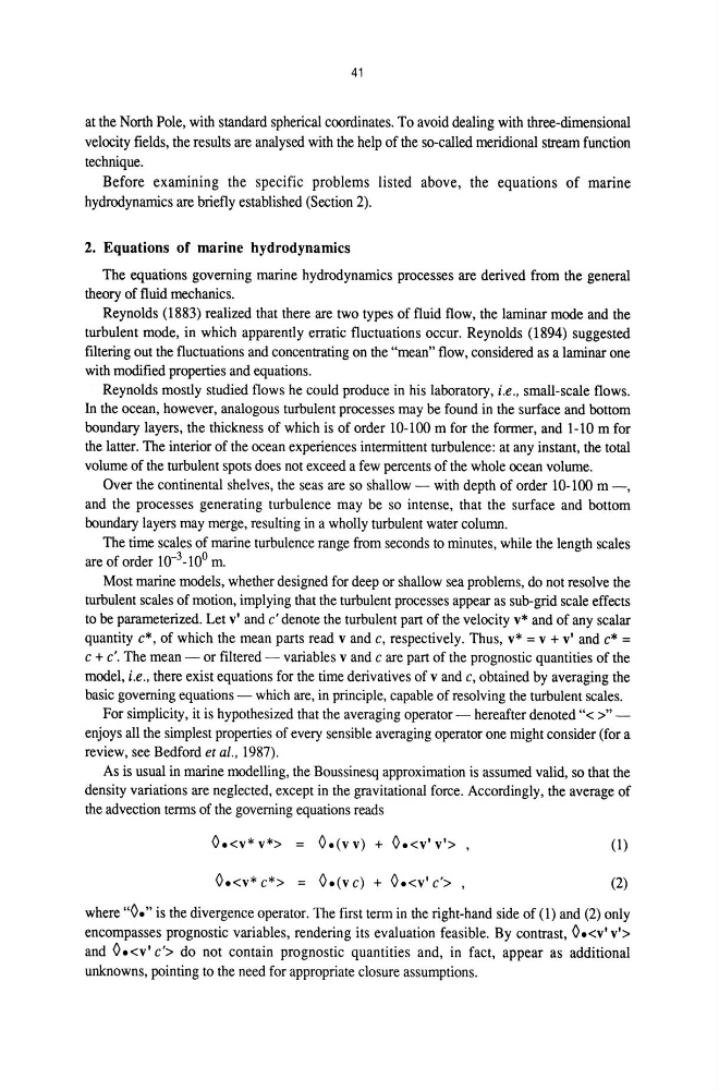
the advection terms of the governing equations reads
O.
O.(v v) + O.
(1)
O.
O.(vc) + O. ,
(2)
where "0." is the divergence operator. The first term in the right-hand side of (1) and (2) only
encompasses prognostic variables, rendering its evaluation feasible. By contrast, O.
and O. do not contain prognostic quantities and, in fact, appear as additional
unknowns, pointing to the need for appropriate closure assumptions.
at the North Pole, with standard spherical coordinates. To avoid dealing with three-dimensional
velocity fields, the results are analysed with the help of the so-called meridional stream function
technique.
Before examining the specific problems listed above, the equations of marine
hydrodynamics are briefly established (Section 2).
2. Equations of marine hydrodynamics
The equations governing marine hydrodynamics processes are derived from the general
theory of fluid mechanics.
Reynolds (1883) realized that there are two types of fluid flow, the laminar mode and the
turbulent mode, in which apparently erratic fluctuations occur. Reynolds (1894) suggested
filtering out the fluctuations and concentrating on the "mean" flow, considered as a laminar one
with modified properties and equations.
Reynolds mostly studied flows he could produce in his laboratory, i.e., small-scale flows.
In the ocean, however, analogous turbulent processes may be found in the surface and bottom
boundary layers, the thickness of which is of order 10-100 m for the former, and 1-10 m for
the latter. The interior of the ocean experiences intermittent turbulence: at any instant, the total
volume of the turbulent spots does not exceed a few percents of the whole ocean volume.
Over the continental shelves, the seas are so shallow - with depth of order 10-100 m-,
and the processes generating turbulence may be so intense, that the surface and bottom
boundary layers may merge, resulting in a wholly turbulent water column.
The time scales of marine turbulence range from seconds to minutes, while the length scales
are of order 10- 3 -10° m.
Most marine models, whether designed for deep or shallow sea problems, do not resolve the
turbulent scales of motion, implying that the turbulent processes appear as sub-grid scale effects
to be parameterized. Let v' and c' denote the turbulent part of the velocity v* and of any scalar
quantity c*, of which the mean parts read v and c, respectively. Thus, v* = v + v' and c* =
c + c'. The mean - or filtered - variables v and c are part of the prognostic quantities of the
model, i.e., there exist equations for the time derivatives of v and c, obtained by averaging the
basic governing equations - which are, in principle, capable of resolving the turbulent scales.
For simplicity, it is hypothesized that the averaging operator - hereafter denoted "< >" -
enjoys all the simplest properties of every sensible averaging operator one might consider (for a
review, see Bedford et ai., 1987).
As is usual in marine modelling, the Boussinesq approximation is assumed valid, so that the
density variations are neglected, except in the gravitational force. Accordingly, the average of
the advection terms of the governing equations reads
O.
O.(v v) + O.
(1)
O.
O.(vc) + O.
(2)
where "0." is the divergence operator. The first term in the right-hand side of (1) and (2) only
encompasses prognostic variables, rendering its evaluation feasible. By contrast, O.
and O.
unknowns, pointing to the need for appropriate closure assumptions.