

374
2.4 Some aspects of shallow water equations
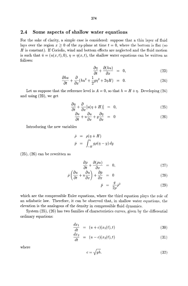
For the sake of clarity, a simple case is considered: suppose that a thin layer of fluid
lays over the region x ~ 0 of the xy-plane at time t = 0, where the bottom is flat (so
H is constant). If Coriolis, wind and bottom effects are neglected and the fluid motion
is such that u = (u( x, t), 0), TJ = TJ( x, t), the shallow water equations can be written as
follows:
0,
o.
(23)
(24)
Let us suppose that the reference level is A = 0, so that h = H +TJ. Developing (24)
and using (23), we get
OTJ a
at + aX [U(TJ + H)]
au
au
OTJ
-+u-+gat
ax
ax
Introducing the new variables
P
p(TJ + H)
0,
o
P
i: gp(TJ - y) dy
(25), (26) can be rewritten as
Op o(pu)
at + ----a;;P (au + u au) + op
at
ax
ax
p
0,
o
9 -2
-P
2p
(25)
(26)
(27)
(28)
(29)
which are the compressible Euler equations, where the third equation plays the role of
an adiabatic law. Therefore, it can be observed that, in shallow water equations, the
elevation is the analogous of the density in compressible fluid dynamics.
System (25), (26) has two families of characteristics curves, given by the differential
ordinary equations:
dXl
(u + C)(Xl(t),t)
(30)
dt
dX2
(u - C)(X2(t), t)
(31)
dt
where
c= [;h.
(32)
2.4 Some aspects of shallow water equations
For the sake of clarity, a simple case is considered: suppose that a thin layer of fluid
lays over the region x ~ 0 of the xy-plane at time t = 0, where the bottom is flat (so
H is constant). If Coriolis, wind and bottom effects are neglected and the fluid motion
is such that u = (u( x, t), 0), TJ = TJ( x, t), the shallow water equations can be written as
follows:
0,
o.
(23)
(24)
Let us suppose that the reference level is A = 0, so that h = H +TJ. Developing (24)
and using (23), we get
OTJ a
at + aX [U(TJ + H)]
au
au
OTJ
-+u-+gat
ax
ax
Introducing the new variables
P
p(TJ + H)
0,
o
P
i: gp(TJ - y) dy
(25), (26) can be rewritten as
Op o(pu)
at + ----a;;P (au + u au) + op
at
ax
ax
p
0,
o
9 -2
-P
2p
(25)
(26)
(27)
(28)
(29)
which are the compressible Euler equations, where the third equation plays the role of
an adiabatic law. Therefore, it can be observed that, in shallow water equations, the
elevation is the analogous of the density in compressible fluid dynamics.
System (25), (26) has two families of characteristics curves, given by the differential
ordinary equations:
dXl
(u + C)(Xl(t),t)
(30)
dt
dX2
(u - C)(X2(t), t)
(31)
dt
where
c= [;h.
(32)