

15
3. Photosynthesis.
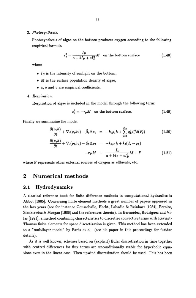
Photosynthesis of algae on the bottom produces oxygen according to the following
empirical formula
s~ =
IB
M on the bottom surface
a + bIB + cI~
(1.48)
where
• IB is the intensity of sunlight on the bottom,
• M is the surface population density of algae,
• a, b and c are empirical coefficients.
4. Respiration.
Respiration of algae is included in the model through the following term:
s~ = -rpM on the bottom surface.
(1.49)
Finally we summarize the model
8(p1h)
-
~ + 'V.(p1hv) - fhD.P1
N.
-k1P1 h + E qfp~;t5(p;)
;=1
(1.50)
8(P2h)
-
~ + 'V·(P2 hv ) - (32D.P2
-rpM +
IB
M+F
a+ bIB + cI'i1
(1.51)
where F represents other external sources of oxygen as efHuents, etc.
2 Numerical methods
2.1 Hydrodynamics
A classical reference book for finite difference methods in computational hydraulics is
Abbot [1985]. Concerning finite element methods a great number of papers appeared in
the last years (see for instance Goussebaile, Hecht, Labadie & Reinhart [1984], Peraire,
Zienkiewicz & Morgan [1986] and the references therein). In Bermudez, Rodriguez and Vilar [1991], a method combining characteristics to discretize convective terms with RaviartThomas finite elements for space discretization is given. This method has been extended
to a "multilayer model" by Pares et al. (see his paper in this proceedings for further
details).
As it is well known, schemes based on (explicit) Euler discretization in time together
with centred differences for flux terms are unconditionally stable for hyperbolic equations even in the linear case. Then upwind discretization should be used. This has been
3. Photosynthesis.
Photosynthesis of algae on the bottom produces oxygen according to the following
empirical formula
s~ =
IB
M on the bottom surface
a + bIB + cI~
(1.48)
where
• IB is the intensity of sunlight on the bottom,
• M is the surface population density of algae,
• a, b and c are empirical coefficients.
4. Respiration.
Respiration of algae is included in the model through the following term:
s~ = -rpM on the bottom surface.
(1.49)
Finally we summarize the model
8(p1h)
-
~ + 'V.(p1hv) - fhD.P1
N.
-k1P1 h + E qfp~;t5(p;)
;=1
(1.50)
8(P2h)
-
~ + 'V·(P2 hv ) - (32D.P2
-rpM +
IB
M+F
a+ bIB + cI'i1
(1.51)
where F represents other external sources of oxygen as efHuents, etc.
2 Numerical methods
2.1 Hydrodynamics
A classical reference book for finite difference methods in computational hydraulics is
Abbot [1985]. Concerning finite element methods a great number of papers appeared in
the last years (see for instance Goussebaile, Hecht, Labadie & Reinhart [1984], Peraire,
Zienkiewicz & Morgan [1986] and the references therein). In Bermudez, Rodriguez and Vilar [1991], a method combining characteristics to discretize convective terms with RaviartThomas finite elements for space discretization is given. This method has been extended
to a "multilayer model" by Pares et al. (see his paper in this proceedings for further
details).
As it is well known, schemes based on (explicit) Euler discretization in time together
with centred differences for flux terms are unconditionally stable for hyperbolic equations even in the linear case. Then upwind discretization should be used. This has been