185
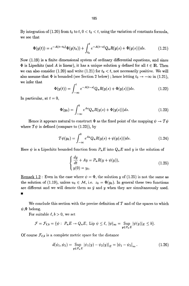
By integration of (1.20) from to to t, 0 < to < t, using the variation of constants formula,
we see that
~(y(t)) = e-A(t-to)~(y(to)) + it e-A(t-S)QnR(y(s) + ~(y(s)))ds.
(1.21)
to
Now (1.19) is a finite dimensional system of ordinary differential equations, and since
~ is Lipschitz (and A is linear), it has a unique solution y defined for all t E JR. Then
we can also consider (1.20) and write (1.21) for to < t, not necessarily positive. We will
also assume that ~ is bounded (see Section 2 below) ; hence letting to -4 -00 in (1.21),
we infer that
eli(y(t)) = [too e-A(t-s)QnR(y(s) + eli(y(s)))ds.
(1.22)
In particular, at t = 0,
(1.23)
Hence it appears natural to construct ~ as the fixed point of the mapping 1/1 -4 T 1/1
where T 1/1 is defined (compare to (1.23)), by
(1.24)
Here 1/1 is a Lipschitz bounded function from PnE into QnE and y is the solution of
{
dy
dt + Ay = PnR(y + 1/1(y)),
y(O) = Yo.
(1.25)
Remark 1.2 : Even in the case where 1/1 = eli, the solution y of (1.25) is not the same as
the solution of (1.19), unless Uo E M, i.e. Zo = eli(yo). In general these two functions
are different and we will denote them as iJ and y when they are simultaneously used .
•
We conclude this section with the precise definition of T and of the spaces to which
1/1, eli belong.
For suitable £, b > 0, we set
:F = :Fl,b = {1/1: PnE -4 QnE, Lip 1jJ :::; £, 11/1100 = Sup 11/1(y)IE:::; b}.
yEPnE
Of course :Fl,b is a complete metric space for the distance
(1.26)