

108
3.2.2.2. Interception and re-evaporation
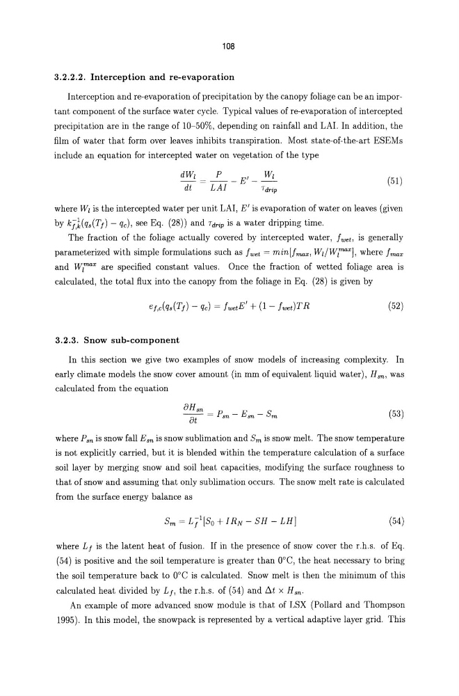
Interception and re-evaporation of precipitation by the canopy foliage can be an important component of the surface water cycle. Typical values of re-evaporation of intercepted
precipitation are in the range of 10-50%, depending on rainfall and LA!. In addition, the
film of water that form over leaves inhibits transpiration. Most state-of-the-art ESEMs
include an equation for intercepted water on vegetation of the type
dWI = ~-E'- WI
dt
LAI
Tdrip
(51)
where WI is the intercepted water per unit LAI, E' is evaporation of water on leaves (given
by kt,l(Qs(T f ) - qc), see Eq. (28)) and Tdrip is a water dripping time.
The fraction of the foliage actually covered by intercepted water, fwet, is generally
parameterized with simple formulations such as fwet = min[fmax, WI/W 1 max ], where fmax
and W I
71WX are specified constant values. Once the fraction of wetted foliage area is
calculated, the total flux into the canopy from the foliage in Eq. (28) is given by
(52)
3.2.3. Snow SUb-component
In this section we give two examples of snow models of increasing complexity. In
early climate models the snow cover amount (in mm of equivalent liquid water), Hsn, was
calculated from the equation
(53)
where P sn is snow fall Esn is snow sublimation and 8m is snow melt. The snow temperature
is not explicitly carried, but it is blended within the temperature calculation of a surface
soil layer by merging snow and soil heat capacities, modifying the surface roughness to
that of snow and assuming that only sublimation occurs. The snow melt rate is calculated
from the surface energy balance as
(54)
where L f is the latent heat of fusion. If in the presence of snow cover the r.h.s. of Eq.
(54) is positive and the soil temperature is greater than DoC, the heat necessary to bring
the soil temperature back to DoC is calculated. Snow melt is then the minimum of this
calculated heat divided by Lf, the r.h.s. of (54) and l':!.t x H sn .
An example of more advanced snow module is that of LSX (Pollard and Thompson
1995). In this model, the snowpack is represented by a vertical adaptive layer grid. This
3.2.2.2. Interception and re-evaporation
Interception and re-evaporation of precipitation by the canopy foliage can be an important component of the surface water cycle. Typical values of re-evaporation of intercepted
precipitation are in the range of 10-50%, depending on rainfall and LA!. In addition, the
film of water that form over leaves inhibits transpiration. Most state-of-the-art ESEMs
include an equation for intercepted water on vegetation of the type
dWI = ~-E'- WI
dt
LAI
Tdrip
(51)
where WI is the intercepted water per unit LAI, E' is evaporation of water on leaves (given
by kt,l(Qs(T f ) - qc), see Eq. (28)) and Tdrip is a water dripping time.
The fraction of the foliage actually covered by intercepted water, fwet, is generally
parameterized with simple formulations such as fwet = min[fmax, WI/W 1 max ], where fmax
and W I
71WX are specified constant values. Once the fraction of wetted foliage area is
calculated, the total flux into the canopy from the foliage in Eq. (28) is given by
(52)
3.2.3. Snow SUb-component
In this section we give two examples of snow models of increasing complexity. In
early climate models the snow cover amount (in mm of equivalent liquid water), Hsn, was
calculated from the equation
(53)
where P sn is snow fall Esn is snow sublimation and 8m is snow melt. The snow temperature
is not explicitly carried, but it is blended within the temperature calculation of a surface
soil layer by merging snow and soil heat capacities, modifying the surface roughness to
that of snow and assuming that only sublimation occurs. The snow melt rate is calculated
from the surface energy balance as
(54)
where L f is the latent heat of fusion. If in the presence of snow cover the r.h.s. of Eq.
(54) is positive and the soil temperature is greater than DoC, the heat necessary to bring
the soil temperature back to DoC is calculated. Snow melt is then the minimum of this
calculated heat divided by Lf, the r.h.s. of (54) and l':!.t x H sn .
An example of more advanced snow module is that of LSX (Pollard and Thompson
1995). In this model, the snowpack is represented by a vertical adaptive layer grid. This