

105
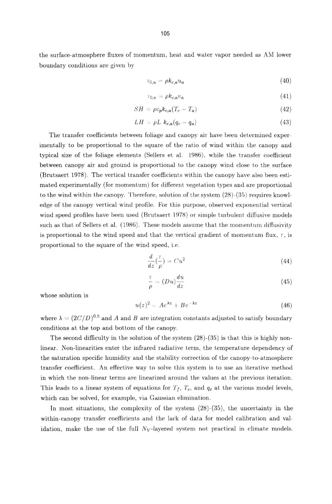
the surface-atmosphere fluxes of momentum, heat and water vapor needed as AM lower
boundary conditions are given by
SH = PCpkc,a(Te - Tal
LH = pL ke,a(qe - qa)
(40)
(41)
(42)
(43)
The transfer coefficients between foliage and canopy air have been determined experimentally to be proportional t.o the square of the ratio of wind within the canopy and
typical size of the foliage elements (Sellers et al. 1986), while the transfer coefficient
between canopy air and ground is proportional to the canopy wind close to the surface
(Brutsaert 1978). The vertical transfer coefficients within the canopy have also been estimated experimentally (for momentum) for different vegetation types and are proportional
to the wind within the canopy. Therefore, solution of the system (28)-(35) requires knowledge of the canopy vertical wind profile. For this purpose, observed exponential vertical
wind speed profiles have been used (Brutsaert 1978) or simple turbulent diffusive models
such as that of Sellers et al. (1986). These models assume that the momentum diffusivity
is proportional to the wind speed and that the vertical gradient of momentum flux, T, is
proportional to the square of the wind speed, i.e.
whose solution is
d T
2
-(-) = Cu
dz p
T
du
- = (Du)p
dz
(44)
(45)
(46)
where A = (2C / D )0.5 and A and B are integration constants adjusted to satisfy boundary
conditions at the top and bottom of the canopy.
The second difficulty in the solution of the system (28)-(35) is that this is highly nonlinear. Non-linearities enter the infrared radiative term, the temperature dependency of
the saturation specific humidity and the stability correction of the canopy-to-atmosphere
transfer coefficient. An effective way to solve this system is to use an iterative method
in which the non-linear terms are linearized around the values at the previous iteration.
This leads to a linear system of equations for If, Te, and qc at the various model levels,
which can be solved, for example, via Gaussian elimination.
In most situations, the complexity of the system (28)-(35), the uncertainty in the
within-canopy transfer coefficients and the lack of data for model calibration and validation, make the use of the full Nv-Iayered system not practical in climate models.
the surface-atmosphere fluxes of momentum, heat and water vapor needed as AM lower
boundary conditions are given by
SH = PCpkc,a(Te - Tal
LH = pL ke,a(qe - qa)
(40)
(41)
(42)
(43)
The transfer coefficients between foliage and canopy air have been determined experimentally to be proportional t.o the square of the ratio of wind within the canopy and
typical size of the foliage elements (Sellers et al. 1986), while the transfer coefficient
between canopy air and ground is proportional to the canopy wind close to the surface
(Brutsaert 1978). The vertical transfer coefficients within the canopy have also been estimated experimentally (for momentum) for different vegetation types and are proportional
to the wind within the canopy. Therefore, solution of the system (28)-(35) requires knowledge of the canopy vertical wind profile. For this purpose, observed exponential vertical
wind speed profiles have been used (Brutsaert 1978) or simple turbulent diffusive models
such as that of Sellers et al. (1986). These models assume that the momentum diffusivity
is proportional to the wind speed and that the vertical gradient of momentum flux, T, is
proportional to the square of the wind speed, i.e.
whose solution is
d T
2
-(-) = Cu
dz p
T
du
- = (Du)p
dz
(44)
(45)
(46)
where A = (2C / D )0.5 and A and B are integration constants adjusted to satisfy boundary
conditions at the top and bottom of the canopy.
The second difficulty in the solution of the system (28)-(35) is that this is highly nonlinear. Non-linearities enter the infrared radiative term, the temperature dependency of
the saturation specific humidity and the stability correction of the canopy-to-atmosphere
transfer coefficient. An effective way to solve this system is to use an iterative method
in which the non-linear terms are linearized around the values at the previous iteration.
This leads to a linear system of equations for If, Te, and qc at the various model levels,
which can be solved, for example, via Gaussian elimination.
In most situations, the complexity of the system (28)-(35), the uncertainty in the
within-canopy transfer coefficients and the lack of data for model calibration and validation, make the use of the full Nv-Iayered system not practical in climate models.