14.3 Solutions
685
and ∇ × H = J +
∂D
∂t
(2)
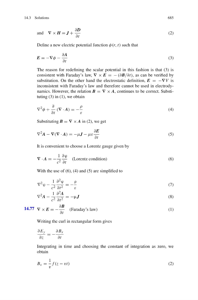
Define a new electric potential function φ(r, t) such that
E = −∇φ −
∂A
∂t
(3)
The reason for redefining the scalar potential in this fashion is that (3) is
consistent with Faraday’s law, ∇ × E = − (∂B/∂t), as can be verified by
substitution. On the other hand the electrostatic definition, E = −∇V is
inconsistent with Faraday’s law and therefore cannot be used in electrodynamics. However, the relation B = ∇ × A, continues to be correct. Substituting (3) in (1), we obtain
∇
2
φ +
∂
∂t
(∇ · A) = −
ρ
ε
(4)
Substituting B = ∇ × A in (2), we get
∇
2 A − ∇(∇ · A) = −μJ − με
∂E
∂t
(5)
It is convenient to choose a Lorentz gauge given by
∇ · A = −
1
c 2
∂ϕ
∂t
(Lorentz condition)
(6)
With the use of (6), (4) and (5) are simplified to
∇
2
ϕ −
1
c 2
∂ 2 ϕ
∂t 2 = −
ρ
ε
(7)
∇
2 A −
1
c 2
∂ 2 A
∂t 2 = −μJ
(8)
14.77 ∇ × E = −
∂B
∂t
(Faraday’s law)
(1)
Writing the curl in rectangular form gives
∂ E y
∂z
= −
∂ B x
∂t
Integrating in time and choosing the constant of integration as zero, we
obtain
B x =
1
v
f (z − vt)
(2)