

240
6 Oscillations
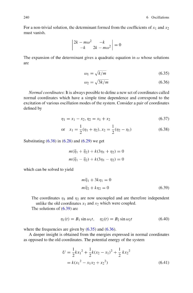
For a non-trivial solution, the determinant formed from the coefficients of x 1 and x 2
must vanish.
2k − mω 2
−k
−k
2k − mω 2
= 0
The expansion of the determinant gives a quadratic equation in ω whose solutions
are
ω 1 =
k/m
(6.35)
ω 2 =
3k/m
(6.36)
Normal coordinates: It is always possible to define a new set of coordinates called
normal coordinates which have a simple time dependence and correspond to the
excitation of various oscillation modes of the system. Consider a pair of coordinates
defined by
η 1 = x 1 − x 2 , η 2 = x 1 + x 2
(6.37)
or x 1 =
1
2
(η 1 + η 2 ), x 2 =
1
2
(η 2 − η 1 )
(6.38)
Substituting (6.38) in (6.28) and (6.29) we get
m( ¨
η 1 + ¨
η 2 ) + k(3η 1 + η 2 ) = 0
m( ¨
η 1 − ¨
η 2 ) + k(3η 1 − η 2 ) = 0
which can be solved to yield
m ¨
η 1 + 3kη 1 = 0
m ¨
η 2 + kη 2 = 0
(6.39)
The coordinates η 1 and η 2 are now uncoupled and are therefore independent
unlike the old coordinates x 1 and x 2 which were coupled.
The solutions of (6.39) are
η 1 (t) = B 1 sin ω 1 t, η 2 (t) = B 2 sin ω 2 t
(6.40)
where the frequencies are given by (6.35) and (6.36).
A deeper insight is obtained from the energies expressed in normal coordinates
as opposed to the old coordinates. The potential energy of the system
U =
1
2
kx 1
2
+
1
2
k(x 2 − x 1 )
2
+
1
2
kx 2
2
= k(x 1
2
− x 1 x 2 + x 2
2
)
(6.41)
6 Oscillations
For a non-trivial solution, the determinant formed from the coefficients of x 1 and x 2
must vanish.
2k − mω 2
−k
−k
2k − mω 2
= 0
The expansion of the determinant gives a quadratic equation in ω whose solutions
are
ω 1 =
k/m
(6.35)
ω 2 =
3k/m
(6.36)
Normal coordinates: It is always possible to define a new set of coordinates called
normal coordinates which have a simple time dependence and correspond to the
excitation of various oscillation modes of the system. Consider a pair of coordinates
defined by
η 1 = x 1 − x 2 , η 2 = x 1 + x 2
(6.37)
or x 1 =
1
2
(η 1 + η 2 ), x 2 =
1
2
(η 2 − η 1 )
(6.38)
Substituting (6.38) in (6.28) and (6.29) we get
m( ¨
η 1 + ¨
η 2 ) + k(3η 1 + η 2 ) = 0
m( ¨
η 1 − ¨
η 2 ) + k(3η 1 − η 2 ) = 0
which can be solved to yield
m ¨
η 1 + 3kη 1 = 0
m ¨
η 2 + kη 2 = 0
(6.39)
The coordinates η 1 and η 2 are now uncoupled and are therefore independent
unlike the old coordinates x 1 and x 2 which were coupled.
The solutions of (6.39) are
η 1 (t) = B 1 sin ω 1 t, η 2 (t) = B 2 sin ω 2 t
(6.40)
where the frequencies are given by (6.35) and (6.36).
A deeper insight is obtained from the energies expressed in normal coordinates
as opposed to the old coordinates. The potential energy of the system
U =
1
2
kx 1
2
+
1
2
k(x 2 − x 1 )
2
+
1
2
kx 2
2
= k(x 1
2
− x 1 x 2 + x 2
2
)
(6.41)