

Position and Displacement
One general way of locating a particle (or particle-like object) is with a position
vector , which is a vector that extends from a reference point (usually the
origin) to the particle. In the unit-vector notation of Module 3-2, can be written
(4-1)
where x , y , and z are the vector components of and the coefficients x, y, and z
are its scalar components.
The coefficients x, y, and z give the particle’s location along the coordinate
axes and relative to the origin; that is, the particle has the rectangular coordinates
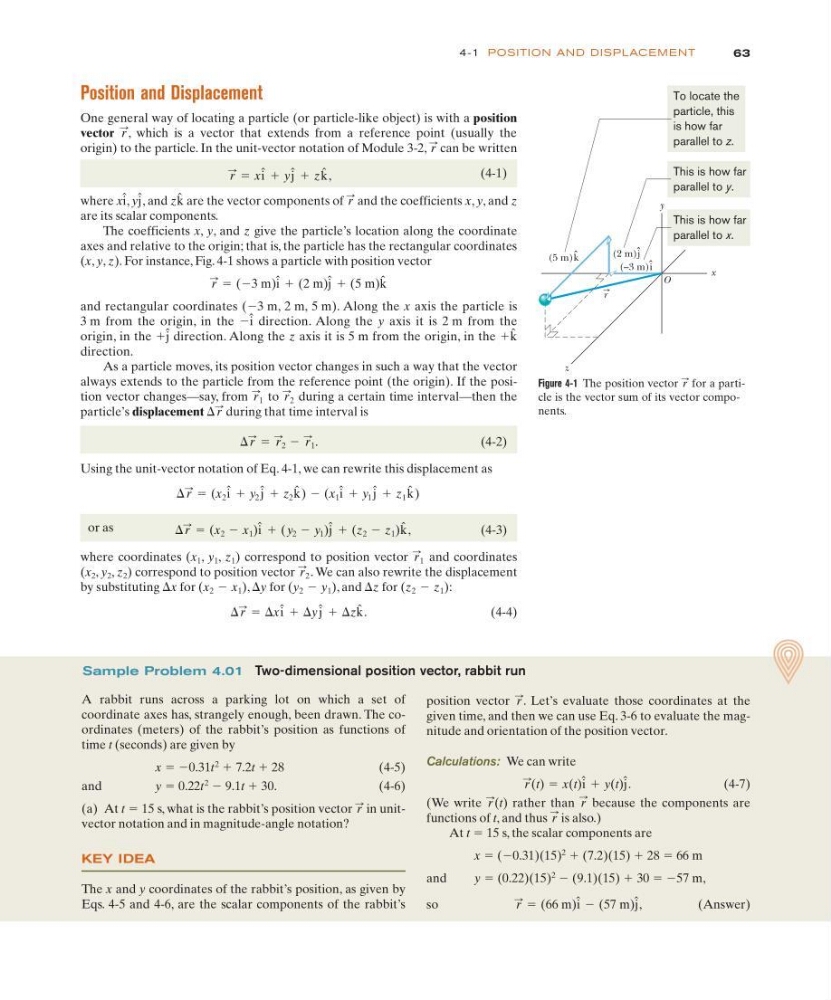
(x, y, z). For instance, Fig. 4-1 shows a particle with position vector
and rectangular coordinates (Ϫ3 m, 2 m, 5 m). Along the x axis the particle is
3 m from the origin, in the
direction. Along the y axis it is 2 m from the
origin, in the
direction. Along the z axis it is 5 m from the origin, in the
direction.
As a particle moves, its position vector changes in such a way that the vector
always extends to the particle from the reference point (the origin). If the position vector changes—say, from
to
during a certain time interval—then the
particle’s displacement
during that time interval is
(4-2)
Using the unit-vector notation of Eq. 4-1, we can rewrite this displacement as
or as
(4-3)
where coordinates (x 1 , y 1 , z 1 ) correspond to position vector
and coordinates
(x 2 , y 2 , z 2 ) correspond to position vector . We can also rewrite the displacement
by substituting x for (x 2 x 1 ), y for (y 2 y 1 ), and z for (z 2 z 1 ):
(4-4)
⌬ r
: ϭ ⌬xi ˆ ϩ ⌬y j ˆ ϩ ⌬zk ˆ .
Ϫ
⌬
Ϫ
⌬
Ϫ
⌬
r
:
2
r
:
1
⌬ r
: ϭ (x 2 Ϫ x 1 )i ˆ ϩ (y 2 Ϫ y 1 )j ˆ ϩ (z 2 Ϫ z 1 )k ˆ ,
⌬ r
: ϭ (x 2 i ˆ ϩ y 2 j ˆ ϩ z 2 k ˆ ) Ϫ (x 1 i ˆ ϩ y 1 j ˆ ϩ z 1 k ˆ )
⌬ r
: ϭ r
:
2 Ϫ r
:
1 .
⌬ r
:
r
:
2
r
:
1
ϩk ˆ
ϩj ˆ
Ϫi ˆ
r
: ϭ (Ϫ3 m)i ˆ ϩ (2 m)j ˆ ϩ (5 m)k ˆ
r
:
k ˆ
j
ˆ
i
ˆ
r
: ϭ xi ˆ ϩ yj ˆ ϩ zk ˆ ,
r
:
r
:
Figure 4-1 The position vector for a particle is the vector sum of its vector components.
r
:
y
x
z
(–3 m)i
(2 m)j
(5 m)k
O
ˆ
ˆ
ˆ
r
To locate the
particle, this
is how far
parallel to z.
This is how far
parallel to y.
This is how far
parallel to x.
position vector . Let’s evaluate those coordinates at the
given time, and then we can use Eq. 3-6 to evaluate the magnitude and orientation of the position vector.
r
:
Sample Problem 4.01 Two-dimensional position vector, rabbit run
A rabbit runs across a parking lot on which a set of
coordinate axes has, strangely enough, been drawn. The coordinates (meters) of the rabbit’s position as functions of
time t (seconds) are given by
x ϭ Ϫ0.31t
2 ϩ 7.2t ϩ 28
(4-5)
and
y ϭ 0.22t
2 Ϫ 9.1t ϩ 30.
(4-6)
(a) At t ϭ 15 s, what is the rabbit’s position vector in unitvector notation and in magnitude-angle notation?
KEY IDEA
The x and y coordinates of the rabbit’s position, as given by
Eqs. 4-5 and 4-6, are the scalar components of the rabbit’s
r
:
Calculations: We can write
(4-7)
(We write
rather than because the components are
functions of t, and thus is also.)
At t ϭ 15 s, the scalar components are
x ϭ (Ϫ0.31)(15)
2 ϩ (7.2)(15) ϩ 28 ϭ 66 m
and
y ϭ (0.22)(15)
2 Ϫ (9.1)(15) ϩ 30 ϭ Ϫ57 m,
so
(Answer)
r
: ϭ (66 m)i ˆ Ϫ (57 m)j ˆ ,
r
:
r
:
r
: (t)
r
: (t) ϭ x(t)i ˆ ϩ y(t)j ˆ .
63
4-1 POSITION AN D DISPL ACE M E NT
One general way of locating a particle (or particle-like object) is with a position
vector , which is a vector that extends from a reference point (usually the
origin) to the particle. In the unit-vector notation of Module 3-2, can be written
(4-1)
where x , y , and z are the vector components of and the coefficients x, y, and z
are its scalar components.
The coefficients x, y, and z give the particle’s location along the coordinate
axes and relative to the origin; that is, the particle has the rectangular coordinates
(x, y, z). For instance, Fig. 4-1 shows a particle with position vector
and rectangular coordinates (Ϫ3 m, 2 m, 5 m). Along the x axis the particle is
3 m from the origin, in the
direction. Along the y axis it is 2 m from the
origin, in the
direction. Along the z axis it is 5 m from the origin, in the
direction.
As a particle moves, its position vector changes in such a way that the vector
always extends to the particle from the reference point (the origin). If the position vector changes—say, from
to
during a certain time interval—then the
particle’s displacement
during that time interval is
(4-2)
Using the unit-vector notation of Eq. 4-1, we can rewrite this displacement as
or as
(4-3)
where coordinates (x 1 , y 1 , z 1 ) correspond to position vector
and coordinates
(x 2 , y 2 , z 2 ) correspond to position vector . We can also rewrite the displacement
by substituting x for (x 2 x 1 ), y for (y 2 y 1 ), and z for (z 2 z 1 ):
(4-4)
⌬ r
: ϭ ⌬xi ˆ ϩ ⌬y j ˆ ϩ ⌬zk ˆ .
Ϫ
⌬
Ϫ
⌬
Ϫ
⌬
r
:
2
r
:
1
⌬ r
: ϭ (x 2 Ϫ x 1 )i ˆ ϩ (y 2 Ϫ y 1 )j ˆ ϩ (z 2 Ϫ z 1 )k ˆ ,
⌬ r
: ϭ (x 2 i ˆ ϩ y 2 j ˆ ϩ z 2 k ˆ ) Ϫ (x 1 i ˆ ϩ y 1 j ˆ ϩ z 1 k ˆ )
⌬ r
: ϭ r
:
2 Ϫ r
:
1 .
⌬ r
:
r
:
2
r
:
1
ϩk ˆ
ϩj ˆ
Ϫi ˆ
r
: ϭ (Ϫ3 m)i ˆ ϩ (2 m)j ˆ ϩ (5 m)k ˆ
r
:
k ˆ
j
ˆ
i
ˆ
r
: ϭ xi ˆ ϩ yj ˆ ϩ zk ˆ ,
r
:
r
:
Figure 4-1 The position vector for a particle is the vector sum of its vector components.
r
:
y
x
z
(–3 m)i
(2 m)j
(5 m)k
O
ˆ
ˆ
ˆ
r
To locate the
particle, this
is how far
parallel to z.
This is how far
parallel to y.
This is how far
parallel to x.
position vector . Let’s evaluate those coordinates at the
given time, and then we can use Eq. 3-6 to evaluate the magnitude and orientation of the position vector.
r
:
Sample Problem 4.01 Two-dimensional position vector, rabbit run
A rabbit runs across a parking lot on which a set of
coordinate axes has, strangely enough, been drawn. The coordinates (meters) of the rabbit’s position as functions of
time t (seconds) are given by
x ϭ Ϫ0.31t
2 ϩ 7.2t ϩ 28
(4-5)
and
y ϭ 0.22t
2 Ϫ 9.1t ϩ 30.
(4-6)
(a) At t ϭ 15 s, what is the rabbit’s position vector in unitvector notation and in magnitude-angle notation?
KEY IDEA
The x and y coordinates of the rabbit’s position, as given by
Eqs. 4-5 and 4-6, are the scalar components of the rabbit’s
r
:
Calculations: We can write
(4-7)
(We write
rather than because the components are
functions of t, and thus is also.)
At t ϭ 15 s, the scalar components are
x ϭ (Ϫ0.31)(15)
2 ϩ (7.2)(15) ϩ 28 ϭ 66 m
and
y ϭ (0.22)(15)
2 Ϫ (9.1)(15) ϩ 30 ϭ Ϫ57 m,
so
(Answer)
r
: ϭ (66 m)i ˆ Ϫ (57 m)j ˆ ,
r
:
r
:
r
: (t)
r
: (t) ϭ x(t)i ˆ ϩ y(t)j ˆ .
63
4-1 POSITION AN D DISPL ACE M E NT