

A Microscopic View of Ohm’s Law
To find out why particular materials obey Ohm’s law, we must look into the
details of the conduction process at the atomic level. Here we consider only conduction in metals, such as copper. We base our analysis on the free-electron
model, in which we assume that the conduction electrons in the metal are free to
move throughout the volume of a sample, like the molecules of a gas in a closed
container. We also assume that the electrons collide not with one another but
only with atoms of the metal.
According to classical physics, the electrons should have a Maxwellian speed distribution somewhat like that of the molecules in a gas (Module 19-6), and thus the average electron speed should depend on the temperature. The motions of electrons
are, however, governed not by the laws of classical physics but by those of quantum
physics. As it turns out, an assumption that is much closer to the quantum reality is
that conduction electrons in a metal move with a single effective speed v eff , and this
speed is essentially independent of the temperature. For copper, v eff Ϸ 1.6 ϫ 10
6
m/s.
When we apply an electric field to a metal sample, the electrons modify their
random motions slightly and drift very slowly — in a direction opposite that of
the field — with an average drift speed v d . The drift speed in a typical metallic
conductor is about 5 ϫ 10
Ϫ7
m/s, less than the effective speed (1.6 ϫ 10
6
m/s) by
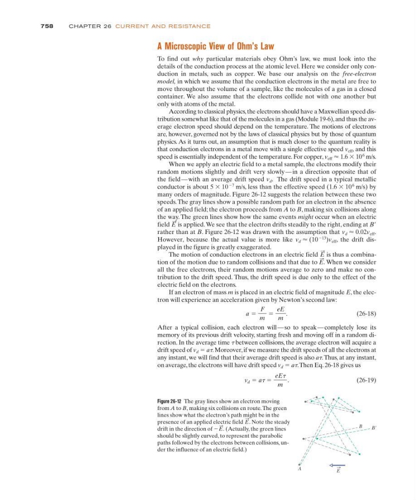
many orders of magnitude. Figure 26-12 suggests the relation between these two
speeds. The gray lines show a possible random path for an electron in the absence
of an applied field; the electron proceeds from A to B, making six collisions along
the way. The green lines show how the same events might occur when an electric
field is applied. We see that the electron drifts steadily to the right, ending at BЈ
rather than at B. Figure 26-12 was drawn with the assumption that v d Ϸ 0.02v eff .
However, because the actual value is more like v d Ϸ (10
Ϫ13
)v eff , the drift displayed in the figure is greatly exaggerated.
The motion of conduction electrons in an electric field is thus a combination of the motion due to random collisions and that due to When we consider
all the free electrons, their random motions average to zero and make no contribution to the drift speed. Thus, the drift speed is due only to the effect of the
electric field on the electrons.
If an electron of mass m is placed in an electric field of magnitude E, the electron will experience an acceleration given by Newton’s second law:
(26-18)
After a typical collision, each electron will — so to speak — completely lose its
memory of its previous drift velocity, starting fresh and moving off in a random direction. In the average time t between collisions, the average electron will acquire a
drift speed of v d ϭ at. Moreover, if we measure the drift speeds of all the electrons at
any instant, we will find that their average drift speed is also at. Thus, at any instant,
on average, the electrons will have drift speed v d ϭ at.Then Eq. 26-18 gives us
(26-19)
v d ϭ at ϭ
eEt
m
.
a ϭ
F
m
ϭ
eE
m
.
E
:
.
E
:
E
:
758
CHAPTE R 26 CU R R E NT AN D R ESISTANCE
B
B'
A
E
Figure 26-12 The gray lines show an electron moving
from A to B, making six collisions en route.The green
lines show what the electron’s path might be in the
presence of an applied electric field Note the steady
drift in the direction of
(Actually, the green lines
should be slightly curved, to represent the parabolic
paths followed by the electrons between collisions, under the influence of an electric field.)
ϪE
: .
E
:
.