699
24-5 POTE NTIAL DU E TO A CONTI N UOUS CHARG E DISTR I B UTION
integrate to sum the potentials due to all the charge elements:
(24-32)
The integral must be taken over the entire charge distribution. Note that because
the electric potential is a scalar, there are no vector components to consider in
Eq. 24-32.
We now examine two continuous charge distributions, a line and a disk.
Line of Charge
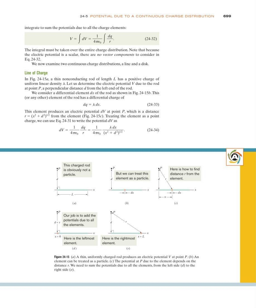
In Fig. 24-15a, a thin nonconducting rod of length L has a positive charge of
uniform linear density l. Let us determine the electric potential V due to the rod
at point P, a perpendicular distance d from the left end of the rod.
We consider a differential element dx of the rod as shown in Fig. 24-15b. This
(or any other) element of the rod has a differential charge of
dq ϭ l dx.
( 2 4 - 3 3 )
This element produces an electric potential dV at point P, which is a distance
r ϭ (x
2 ϩ d
2
)
1/2
from the element (Fig. 24-15c). Treating the element as a point
charge, we can use Eq. 24-31 to write the potential dV as
(24-34)
dV ϭ
1
4p´ 0
dq
r
ϭ
1
4p´ 0
l dx
(x
2 ϩ d
2
)
1/2
.
V ϭ ͵dV ϭ
1
4p´ 0
͵
dq
r
.
(b)
d
P
x
dx
L
d
P
x
(a)
d = r
P
x
(d )
(c)
x
d
P
x
dx
r
x = 0
d
r
P
x
(e )
x = L
This charged rod
is obviously not a
particle.
Our job is to add the
potentials due to all
the elements.
Here is the leftmost
element.
Here is the rightmost
element.
But we can treat this
element as a particle.
Here is how to find
distance r from the
element.
Figure 24-15 (a) A thin, uniformly charged rod produces an electric potential V at point P. (b) An
element can be treated as a particle. (c) The potential at P due to the element depends on the
distance r. We need to sum the potentials due to all the elements, from the left side (d) to the
right side (e).
A