

661
23-1 ELECTRIC FLUX
An inward piercing field is negative flux. An outward piercing field is positive
flux. A skimming field is zero flux.
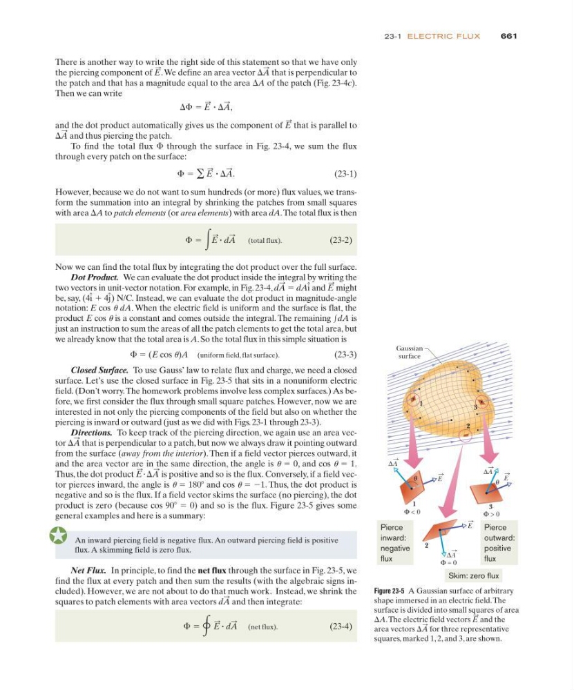
Net Flux. In principle, to find the net flux through the surface in Fig. 23-5, we
find the flux at every patch and then sum the results (with the algebraic signs included). However, we are not about to do that much work. Instead, we shrink the
squares to patch elements with area vectors
and then integrate:
(net flux).
(23-4)
⌽ ϭ ͶE
: ؒ dA
:
dA
:
There is another way to write the right side of this statement so that we have only
the piercing component of .We define an area vector
that is perpendicular to
the patch and that has a magnitude equal to the area ⌬A of the patch (Fig. 23-4c).
Then we can write
and the dot product automatically gives us the component of that is parallel to
and thus piercing the patch.
To find the total flux ⌽ through the surface in Fig. 23-4, we sum the flux
through every patch on the surface:
(23-1)
However, because we do not want to sum hundreds (or more) flux values, we transform the summation into an integral by shrinking the patches from small squares
with area ⌬A to patch elements (or area elements) with area dA.The total flux is then
(total flux).
(23-2)
Now we can find the total flux by integrating the dot product over the full surface.
Dot Product. We can evaluate the dot product inside the integral by writing the
two vectors in unit-vector notation. For example, in Fig. 23-4,
ϭ dA and might
E
:
i
ˆ
dA
:
⌽ ϭ ͵E
: ؒ dA
:
⌽ ϭ ͚ E
: ؒ ⌬A
: .
⌬A
:
E
:
⌬⌽ ϭ E
: ؒ ⌬A
: ,
⌬A
:
E
:
notation: E cos u dA. When the electric field is uniform and the surface is flat, the
product E cos u is a constant and comes outside the integral. The remaining
is
just an instruction to sum the areas of all the patch elements to get the total area, but
we already know that the total area is A. So the total flux in this simple situation is
⌽ ϭ (E cos u)A (uniform field, flat surface).
(23-3)
Closed Surface. To use Gauss’ law to relate flux and charge, we need a closed
surface. Let’s use the closed surface in Fig. 23-5 that sits in a nonuniform electric
field. (Don’t worry.The homework problems involve less complex surfaces.) As before, we first consider the flux through small square patches. However, now we are
interested in not only the piercing components of the field but also on whether the
piercing is inward or outward (just as we did with Figs. 23-1 through 23-3).
Directions. To keep track of the piercing direction, we again use an area vector
that is perpendicular to a patch, but now we always draw it pointing outward
from the surface (away from the interior). Then if a field vector pierces outward, it
and the area vector are in the same direction, the angle is u ϭ 0, and cos u ϭ 1.
Thus, the dot product
is positive and so is the flux. Conversely, if a field vector pierces inward, the angle is u ϭ 180Њ and cos u ϭ Ϫ1. Thus, the dot product is
negative and so is the flux. If a field vector skims the surface (no piercing), the dot
product is zero (because cos 90Њ ϭ 0) and so is the flux. Figure 23-5 gives some
general examples and here is a summary:
⌬A
:
E
: и
⌬A
:
͵dA
Gaussian
surface
1
3
2
∆
θ
1
Φ < 0
Φ = 0
Φ > 0
3
θ
2
A
∆ A
∆ A
E
E
E
Pierce
inward:
negative
flux
Pierce
outward:
positive
flux
Skim: zero flux
Figure 23-5 A Gaussian surface of arbitrary
shape immersed in an electric field. The
surface is divided into small squares of area
⌬A.The electric field vectors and the
area vectors
for three representative
squares, marked 1, 2, and 3, are shown.
⌬A
:
E
:
be, say, (4 ϩ 4 ) N/C. Instead, we can evaluate the dot product in magnitude-angle
j
ˆ
i
ˆ