

600
CHAPTE R 20 ENTROPY AND THE SECOND LAW OF THERMODYNAM ICS
You should verify the multiplicities for all the configurations in Table 20-1.
The basic assumption of statistical mechanics is that
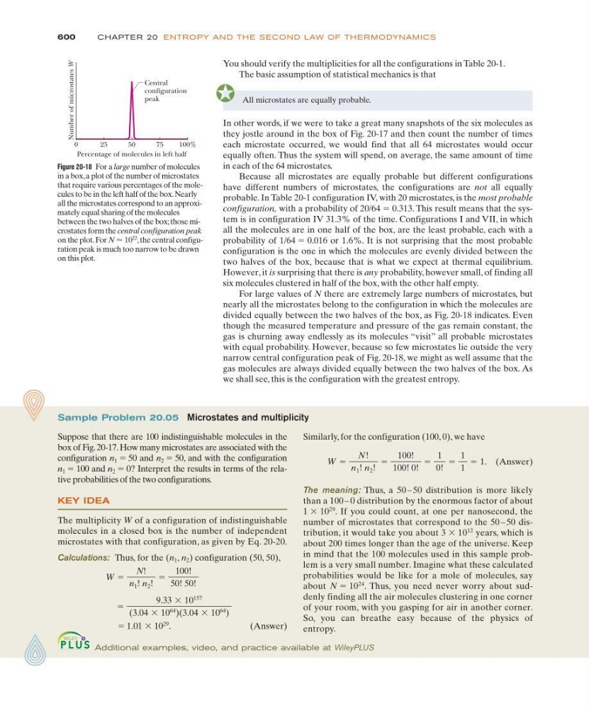
Figure 20-18 For a large number of molecules
in a box, a plot of the number of microstates
that require various percentages of the molecules to be in the left half of the box. Nearly
all the microstates correspond to an approximately equal sharing of the molecules
between the two halves of the box; those microstates form the central configuration peak
on the plot. For N Ϸ 10
22
,the central configuration peak is much too narrow to be drawn
on this plot.
0
25
50
75
100%
Number of microstates
W
Percentage of molecules in left half
Central
configuration
peak
All microstates are equally probable.
In other words, if we were to take a great many snapshots of the six molecules as
they jostle around in the box of Fig. 20-17 and then count the number of times
each microstate occurred, we would find that all 64 microstates would occur
equally often. Thus the system will spend, on average, the same amount of time
in each of the 64 microstates.
Because all microstates are equally probable but different configurations
have different numbers of microstates, the configurations are not all equally
probable. In Table 20-1 configuration IV, with 20 microstates, is the most probable
configuration, with a probability of 20/64 ϭ 0.313. This result means that the system is in configuration IV 31.3% of the time. Configurations I and VII, in which
all the molecules are in one half of the box, are the least probable, each with a
probability of 1/64 ϭ 0.016 or 1.6%. It is not surprising that the most probable
configuration is the one in which the molecules are evenly divided between the
two halves of the box, because that is what we expect at thermal equilibrium.
However, it is surprising that there is any probability, however small, of finding all
six molecules clustered in half of the box, with the other half empty.
For large values of N there are extremely large numbers of microstates, but
nearly all the microstates belong to the configuration in which the molecules are
divided equally between the two halves of the box, as Fig. 20-18 indicates. Even
though the measured temperature and pressure of the gas remain constant, the
gas is churning away endlessly as its molecules “visit” all probable microstates
with equal probability. However, because so few microstates lie outside the very
narrow central configuration peak of Fig. 20-18, we might as well assume that the
gas molecules are always divided equally between the two halves of the box. As
we shall see, this is the configuration with the greatest entropy.
Similarly, for the configuration (100, 0), we have
(Answer)
The meaning: Thus, a 50 – 50 distribution is more likely
than a 100 – 0 distribution by the enormous factor of about
1 ϫ 10
29
. If you could count, at one per nanosecond, the
number of microstates that correspond to the 50 – 50 distribution, it would take you about 3 ϫ 10
12
years, which is
about 200 times longer than the age of the universe. Keep
in mind that the 100 molecules used in this sample problem is a very small number. Imagine what these calculated
probabilities would be like for a mole of molecules, say
about N ϭ 10
24
. Thus, you need never worry about suddenly finding all the air molecules clustering in one corner
of your room, with you gasping for air in another corner.
So, you can breathe easy because of the physics of
entropy.
W ϭ
N!
n 1 ! n 2 !
ϭ
100!
100! 0!
ϭ
1
0!
ϭ
1
1
ϭ 1.
Sample Problem 20.05 Microstates and multiplicity
Suppose that there are 100 indistinguishable molecules in the
box of Fig. 20-17. How many microstates are associated with the
configuration n 1 ϭ 50 and n 2 ϭ 50, and with the configuration
n 1 ϭ 100 and n 2 ϭ 0? Interpret the results in terms of the relative probabilities of the two configurations.
KEY IDEA
The multiplicity W of a configuration of indistinguishable
molecules in a closed box is the number of independent
microstates with that configuration, as given by Eq. 20-20.
Calculations: Thus, for the (n 1 , n 2 ) configuration (50, 50),
ϭ 1.01 ϫ 10
29
.
( A n s w e r )
ϭ
9.33 ϫ 10
157
(3.04 ϫ 10
64
)(3.04 ϫ 10
64
)
W ϭ
N!
n 1 ! n 2 !
ϭ
100!
50! 50!
Additional examples, video, and practice available at WileyPLUS