

497
17-6 BEATS
Beats
If we listen, a few minutes apart, to two sounds whose frequencies are, say, 552
and 564 Hz, most of us cannot tell one from the other because the frequencies are
so close to each other. However, if the sounds reach our ears simultaneously,
what we hear is a sound whose frequency is 558 Hz, the average of the two combining frequencies. We also hear a striking variation in the intensity of this
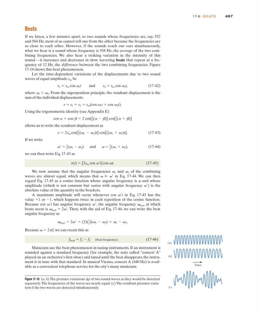
sound — it increases and decreases in slow, wavering beats that repeat at a frequency of 12 Hz, the difference between the two combining frequencies. Figure
17-18 shows this beat phenomenon.
Let the time-dependent variations of the displacements due to two sound
waves of equal amplitude s m be
s 1 ϭ s m cos v 1 t
and
s 2 ϭ s m cos v 2 t,
( 1 7 - 4 2 )
where v 1 Ͼ v 2 . From the superposition principle, the resultant displacement is the
sum of the individual displacements:
s ϭ s 1 ϩ s 2 ϭ s m (cos v 1 t ϩ cos v 2 t).
Using the trigonometric identity (see Appendix E)
allows us to write the resultant displacement as
.
( 1 7 - 4 3 )
If we write
vЈ ϭ (v 1 Ϫ v 2 ) and
v ϭ (v 1 ϩ v 2 ),
(17-44)
we can then write Eq. 17-43 as
s(t) ϭ [2s m cos vЈt] cos vt.
(17-45)
We now assume that the angular frequencies v 1 and v 2 of the combining
waves are almost equal, which means that v ӷ vЈ in Eq. 17-44. We can then
regard Eq. 17-45 as a cosine function whose angular frequency is v and whose
amplitude (which is not constant but varies with angular frequency vЈ) is the
absolute value of the quantity in the brackets.
A maximum amplitude will occur whenever cos vЈt in Eq. 17-45 has the
value ϩ1 or Ϫ1, which happens twice in each repetition of the cosine function.
Because cos vЈt has angular frequency vЈ, the angular frequency v beat at which
beats occur is v beat ϭ 2vЈ. Then, with the aid of Eq. 17-44, we can write the beat
angular frequency as
.
Because v ϭ 2pf, we can recast this as
f beat ϭ f 1 Ϫ f 2 (beat frequency).
( 1 7 - 4 6 )
Musicians use the beat phenomenon in tuning instruments. If an instrument is
sounded against a standard frequency (for example, the note called “concert A”
played on an orchestra’s first oboe) and tuned until the beat disappears, the instrument is in tune with that standard. In musical Vienna, concert A (440 Hz) is available as a convenient telephone service for the city’s many musicians.
v beat ϭ 2vЈ ϭ (2)(
1
2 )(v 1 Ϫ v 2 ) ϭ v 1 Ϫ v 2
1
2
1
2
s ϭ 2 s m cos[
1
2 (v 1 Ϫ v 2 )t] cos[
1
2 (v 1 ϩ v 2 )t]
cos a ϩ cos b ϭ 2 cos[
1
2 (a Ϫ b)] cos[
1
2 (a ϩ b)]
Figure 17-18 (a, b) The pressure variations ⌬p of two sound waves as they would be detected
separately. The frequencies of the waves are nearly equal. (c) The resultant pressure variation if the two waves are detected simultaneously.
Time
(c)
(b)
(a)
17-6 BEATS
Beats
If we listen, a few minutes apart, to two sounds whose frequencies are, say, 552
and 564 Hz, most of us cannot tell one from the other because the frequencies are
so close to each other. However, if the sounds reach our ears simultaneously,
what we hear is a sound whose frequency is 558 Hz, the average of the two combining frequencies. We also hear a striking variation in the intensity of this
sound — it increases and decreases in slow, wavering beats that repeat at a frequency of 12 Hz, the difference between the two combining frequencies. Figure
17-18 shows this beat phenomenon.
Let the time-dependent variations of the displacements due to two sound
waves of equal amplitude s m be
s 1 ϭ s m cos v 1 t
and
s 2 ϭ s m cos v 2 t,
( 1 7 - 4 2 )
where v 1 Ͼ v 2 . From the superposition principle, the resultant displacement is the
sum of the individual displacements:
s ϭ s 1 ϩ s 2 ϭ s m (cos v 1 t ϩ cos v 2 t).
Using the trigonometric identity (see Appendix E)
allows us to write the resultant displacement as
.
( 1 7 - 4 3 )
If we write
vЈ ϭ (v 1 Ϫ v 2 ) and
v ϭ (v 1 ϩ v 2 ),
(17-44)
we can then write Eq. 17-43 as
s(t) ϭ [2s m cos vЈt] cos vt.
(17-45)
We now assume that the angular frequencies v 1 and v 2 of the combining
waves are almost equal, which means that v ӷ vЈ in Eq. 17-44. We can then
regard Eq. 17-45 as a cosine function whose angular frequency is v and whose
amplitude (which is not constant but varies with angular frequency vЈ) is the
absolute value of the quantity in the brackets.
A maximum amplitude will occur whenever cos vЈt in Eq. 17-45 has the
value ϩ1 or Ϫ1, which happens twice in each repetition of the cosine function.
Because cos vЈt has angular frequency vЈ, the angular frequency v beat at which
beats occur is v beat ϭ 2vЈ. Then, with the aid of Eq. 17-44, we can write the beat
angular frequency as
.
Because v ϭ 2pf, we can recast this as
f beat ϭ f 1 Ϫ f 2 (beat frequency).
( 1 7 - 4 6 )
Musicians use the beat phenomenon in tuning instruments. If an instrument is
sounded against a standard frequency (for example, the note called “concert A”
played on an orchestra’s first oboe) and tuned until the beat disappears, the instrument is in tune with that standard. In musical Vienna, concert A (440 Hz) is available as a convenient telephone service for the city’s many musicians.
v beat ϭ 2vЈ ϭ (2)(
1
2 )(v 1 Ϫ v 2 ) ϭ v 1 Ϫ v 2
1
2
1
2
s ϭ 2 s m cos[
1
2 (v 1 Ϫ v 2 )t] cos[
1
2 (v 1 ϩ v 2 )t]
cos a ϩ cos b ϭ 2 cos[
1
2 (a Ϫ b)] cos[
1
2 (a ϩ b)]
Figure 17-18 (a, b) The pressure variations ⌬p of two sound waves as they would be detected
separately. The frequencies of the waves are nearly equal. (c) The resultant pressure variation if the two waves are detected simultaneously.
Time
(c)
(b)
(a)