

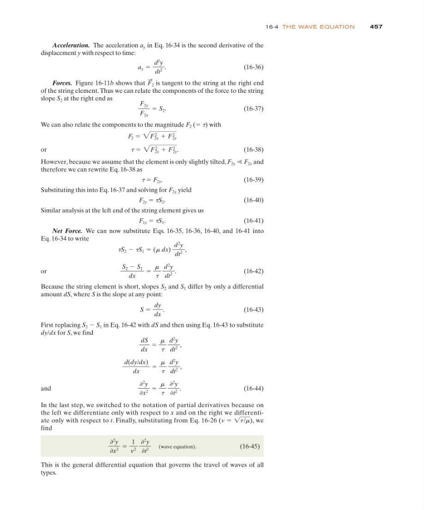
457
16-4 TH E WAVE EQUATION
Acceleration. The acceleration a y in Eq. 16-34 is the second derivative of the
displacement y with respect to time:
(16-36)
Forces. Figure 16-11b shows that 2 is tangent to the string at the right end
of the string element. Thus we can relate the components of the force to the string
slope S 2 at the right end as
(16-37)
We can also relate the components to the magnitude F 2 (ϭ t) with
or
(16-38)
However, because we assume that the element is only slightly tilted, F 2y Ӷ F 2x and
therefore we can rewrite Eq. 16-38 as
t ϭ F 2x .
( 1 6 - 3 9 )
Substituting this into Eq. 16-37 and solving for F 2y yield
F 2y ϭ tS 2 .
( 1 6 - 4 0 )
Similar analysis at the left end of the string element gives us
F 1y ϭ tS 1 .
( 1 6 - 4 1 )
Net Force. We can now substitute Eqs. 16-35, 16-36, 16-40, and 16-41 into
Eq. 16-34 to write
or
(16-42)
Because the string element is short, slopes S 2 and S 1 differ by only a differential
amount dS, where S is the slope at any point:
(16-43)
First replacing S 2 Ϫ S 1 in Eq. 16-42 with dS and then using Eq. 16-43 to substitute
dy/dx for S, we find
and
.
(16-44)
In the last step, we switched to the notation of partial derivatives because on
the left we differentiate only with respect to x and on the right we differentiate only with respect to t. Finally, substituting from Eq. 16-26 (v ϭ
), we
find
(wave equation).
(16-45)
This is the general differential equation that governs the travel of waves of all
types.
≠
2
y
≠x
2
ϭ
1
v
2
≠
2
y
≠t
2
1t /m
≠
2
y
≠x
2
ϭ
m
t
≠
2
y
≠t
2
d(dy/dx)
dx
ϭ
m
t
d
2
y
dt
2
,
dS
dx
ϭ
m
t
d
2
y
dt
2
,
S ϭ
dy
dx
.
S 2 Ϫ S 1
dx
ϭ
m
t
d
2
y
dt
2
.
tS 2 Ϫ tS 1 ϭ (m dx)
d
2
y
dt
2
,
t ϭ 2F
2
2x ϩ F
2
2y .
F 2 ϭ 2F
2
2x ϩ F
2
2y
F 2y
F 2x
ϭ S 2 .
F
:
a y ϭ
d
2
y
dt
2
.
16-4 TH E WAVE EQUATION
Acceleration. The acceleration a y in Eq. 16-34 is the second derivative of the
displacement y with respect to time:
(16-36)
Forces. Figure 16-11b shows that 2 is tangent to the string at the right end
of the string element. Thus we can relate the components of the force to the string
slope S 2 at the right end as
(16-37)
We can also relate the components to the magnitude F 2 (ϭ t) with
or
(16-38)
However, because we assume that the element is only slightly tilted, F 2y Ӷ F 2x and
therefore we can rewrite Eq. 16-38 as
t ϭ F 2x .
( 1 6 - 3 9 )
Substituting this into Eq. 16-37 and solving for F 2y yield
F 2y ϭ tS 2 .
( 1 6 - 4 0 )
Similar analysis at the left end of the string element gives us
F 1y ϭ tS 1 .
( 1 6 - 4 1 )
Net Force. We can now substitute Eqs. 16-35, 16-36, 16-40, and 16-41 into
Eq. 16-34 to write
or
(16-42)
Because the string element is short, slopes S 2 and S 1 differ by only a differential
amount dS, where S is the slope at any point:
(16-43)
First replacing S 2 Ϫ S 1 in Eq. 16-42 with dS and then using Eq. 16-43 to substitute
dy/dx for S, we find
and
.
(16-44)
In the last step, we switched to the notation of partial derivatives because on
the left we differentiate only with respect to x and on the right we differentiate only with respect to t. Finally, substituting from Eq. 16-26 (v ϭ
), we
find
(wave equation).
(16-45)
This is the general differential equation that governs the travel of waves of all
types.
≠
2
y
≠x
2
ϭ
1
v
2
≠
2
y
≠t
2
1t /m
≠
2
y
≠x
2
ϭ
m
t
≠
2
y
≠t
2
d(dy/dx)
dx
ϭ
m
t
d
2
y
dt
2
,
dS
dx
ϭ
m
t
d
2
y
dt
2
,
S ϭ
dy
dx
.
S 2 Ϫ S 1
dx
ϭ
m
t
d
2
y
dt
2
.
tS 2 Ϫ tS 1 ϭ (m dx)
d
2
y
dt
2
,
t ϭ 2F
2
2x ϩ F
2
2y .
F 2 ϭ 2F
2
2x ϩ F
2
2y
F 2y
F 2x
ϭ S 2 .
F
:
a y ϭ
d
2
y
dt
2
.