

448
CHAPTE R 16 WAVES—I
Period, Angular Frequency, and Frequency
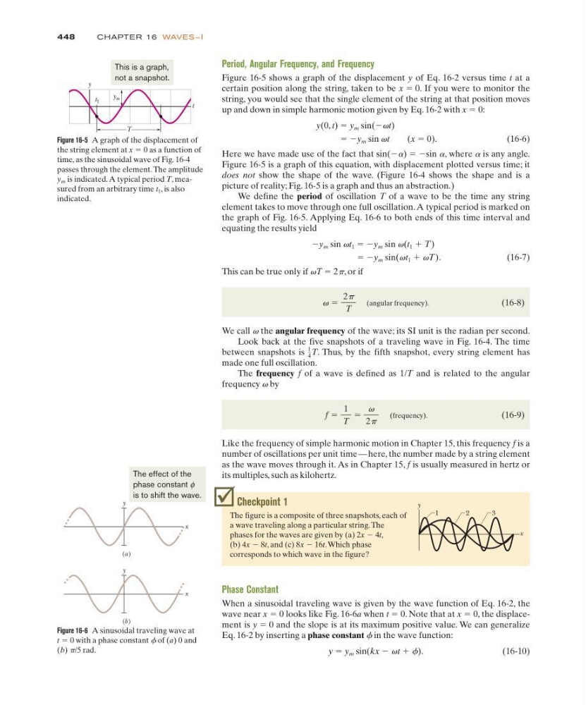
Figure 16-5 shows a graph of the displacement y of Eq. 16-2 versus time t at a
certain position along the string, taken to be x ϭ 0. If you were to monitor the
string, you would see that the single element of the string at that position moves
up and down in simple harmonic motion given by Eq. 16-2 with x ϭ 0:
y(0, t) ϭ y m sin(Ϫvt)
ϭ Ϫy m sin vt
(x ϭ 0).
(16-6)
Here we have made use of the fact that sin(Ϫa) ϭ Ϫsin a, where a is any angle.
Figure 16-5 is a graph of this equation, with displacement plotted versus time; it
does not show the shape of the wave. (Figure 16-4 shows the shape and is a
picture of reality; Fig. 16-5 is a graph and thus an abstraction.)
We define the period of oscillation T of a wave to be the time any string
element takes to move through one full oscillation. A typical period is marked on
the graph of Fig. 16-5. Applying Eq. 16-6 to both ends of this time interval and
equating the results yield
Ϫy m sin vt 1 ϭ Ϫy m sin v(t 1 ϩ T )
ϭ Ϫy m sin(vt 1 ϩ vT ).
(16-7)
This can be true only if vT ϭ 2p, or if
(angular frequency).
(16-8)
We call v the angular frequency of the wave; its SI unit is the radian per second.
Look back at the five snapshots of a traveling wave in Fig. 16-4. The time
between snapshots is T. Thus, by the fifth snapshot, every string element has
made one full oscillation.
The frequency f of a wave is defined as 1/T and is related to the angular
frequency v by
(frequency).
(16-9)
Like the frequency of simple harmonic motion in Chapter 15, this frequency f is a
number of oscillations per unit time — here, the number made by a string element
as the wave moves through it. As in Chapter 15, f is usually measured in hertz or
its multiples, such as kilohertz.
f ϭ
1
T
ϭ
v
2p
1
4
v ϭ
2p
T
Checkpoint 1
The figure is a composite of three snapshots, each of
a wave traveling along a particular string. The
phases for the waves are given by (a) 2x Ϫ 4t,
(b) 4x Ϫ 8t, and (c) 8x Ϫ 16t.Which phase
corresponds to which wave in the figure?
1
2
3
x
y
Figure 16-5 A graph of the displacement of
the string element at x ϭ 0 as a function of
time, as the sinusoidal wave of Fig. 16-4
passes through the element. The amplitude
y m is indicated. A typical period T, measured from an arbitrary time t 1 , is also
indicated.
t
y
t 1
y m
T
This is a graph,
not a snapshot.
Phase Constant
When a sinusoidal traveling wave is given by the wave function of Eq. 16-2, the
wave near x ϭ 0 looks like Fig. 16-6a when t ϭ 0. Note that at x ϭ 0, the displacement is y ϭ 0 and the slope is at its maximum positive value. We can generalize
Eq. 16-2 by inserting a phase constant f in the wave function:
y ϭ y m sin(kx Ϫ vt ϩ f).
(16-10)
Figure 16-6 A sinusoidal traveling wave at
t ϭ 0 with a phase constant f of (a) 0 and
(b) p/5 rad.
x
x
y
y
(a)
(b)
The effect of the
phase constant
is to shift the wave.
φ
CHAPTE R 16 WAVES—I
Period, Angular Frequency, and Frequency
Figure 16-5 shows a graph of the displacement y of Eq. 16-2 versus time t at a
certain position along the string, taken to be x ϭ 0. If you were to monitor the
string, you would see that the single element of the string at that position moves
up and down in simple harmonic motion given by Eq. 16-2 with x ϭ 0:
y(0, t) ϭ y m sin(Ϫvt)
ϭ Ϫy m sin vt
(x ϭ 0).
(16-6)
Here we have made use of the fact that sin(Ϫa) ϭ Ϫsin a, where a is any angle.
Figure 16-5 is a graph of this equation, with displacement plotted versus time; it
does not show the shape of the wave. (Figure 16-4 shows the shape and is a
picture of reality; Fig. 16-5 is a graph and thus an abstraction.)
We define the period of oscillation T of a wave to be the time any string
element takes to move through one full oscillation. A typical period is marked on
the graph of Fig. 16-5. Applying Eq. 16-6 to both ends of this time interval and
equating the results yield
Ϫy m sin vt 1 ϭ Ϫy m sin v(t 1 ϩ T )
ϭ Ϫy m sin(vt 1 ϩ vT ).
(16-7)
This can be true only if vT ϭ 2p, or if
(angular frequency).
(16-8)
We call v the angular frequency of the wave; its SI unit is the radian per second.
Look back at the five snapshots of a traveling wave in Fig. 16-4. The time
between snapshots is T. Thus, by the fifth snapshot, every string element has
made one full oscillation.
The frequency f of a wave is defined as 1/T and is related to the angular
frequency v by
(frequency).
(16-9)
Like the frequency of simple harmonic motion in Chapter 15, this frequency f is a
number of oscillations per unit time — here, the number made by a string element
as the wave moves through it. As in Chapter 15, f is usually measured in hertz or
its multiples, such as kilohertz.
f ϭ
1
T
ϭ
v
2p
1
4
v ϭ
2p
T
Checkpoint 1
The figure is a composite of three snapshots, each of
a wave traveling along a particular string. The
phases for the waves are given by (a) 2x Ϫ 4t,
(b) 4x Ϫ 8t, and (c) 8x Ϫ 16t.Which phase
corresponds to which wave in the figure?
1
2
3
x
y
Figure 16-5 A graph of the displacement of
the string element at x ϭ 0 as a function of
time, as the sinusoidal wave of Fig. 16-4
passes through the element. The amplitude
y m is indicated. A typical period T, measured from an arbitrary time t 1 , is also
indicated.
t
y
t 1
y m
T
This is a graph,
not a snapshot.
Phase Constant
When a sinusoidal traveling wave is given by the wave function of Eq. 16-2, the
wave near x ϭ 0 looks like Fig. 16-6a when t ϭ 0. Note that at x ϭ 0, the displacement is y ϭ 0 and the slope is at its maximum positive value. We can generalize
Eq. 16-2 by inserting a phase constant f in the wave function:
y ϭ y m sin(kx Ϫ vt ϩ f).
(16-10)
Figure 16-6 A sinusoidal traveling wave at
t ϭ 0 with a phase constant f of (a) 0 and
(b) p/5 rad.
x
x
y
y
(a)
(b)
The effect of the
phase constant
is to shift the wave.
φ