

447
16-1 TRANSVE RSE WAVES
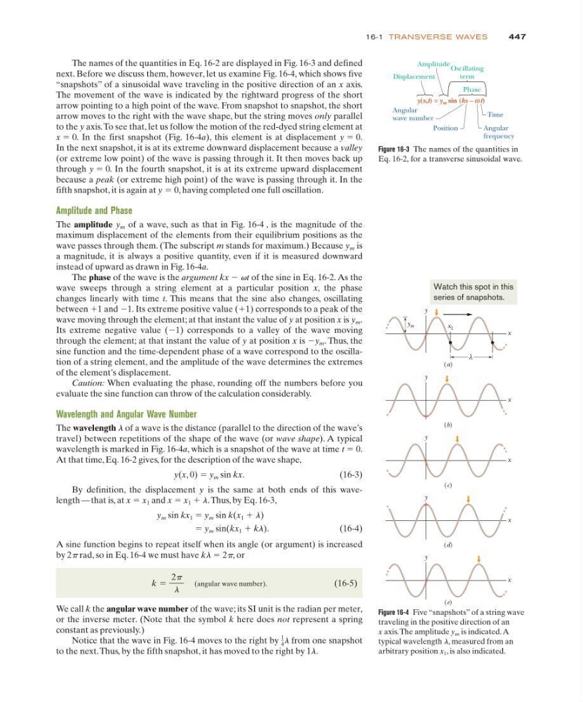
The names of the quantities in Eq. 16-2 are displayed in Fig. 16-3 and defined
next. Before we discuss them, however, let us examine Fig. 16-4, which shows five
“snapshots” of a sinusoidal wave traveling in the positive direction of an x axis.
The movement of the wave is indicated by the rightward progress of the short
arrow pointing to a high point of the wave. From snapshot to snapshot, the short
arrow moves to the right with the wave shape, but the string moves only parallel
to the y axis. To see that, let us follow the motion of the red-dyed string element at
x ϭ 0. In the first snapshot (Fig. 16-4a), this element is at displacement y ϭ 0.
In the next snapshot, it is at its extreme downward displacement because a valley
(or extreme low point) of the wave is passing through it. It then moves back up
through y ϭ 0. In the fourth snapshot, it is at its extreme upward displacement
because a peak (or extreme high point) of the wave is passing through it. In the
fifth snapshot, it is again at y ϭ 0, having completed one full oscillation.
Amplitude and Phase
The amplitude y m of a wave, such as that in Fig. 16-4 , is the magnitude of the
maximum displacement of the elements from their equilibrium positions as the
wave passes through them. (The subscript m stands for maximum.) Because y m is
a magnitude, it is always a positive quantity, even if it is measured downward
instead of upward as drawn in Fig. 16-4a.
The phase of the wave is the argument kx Ϫ vt of the sine in Eq. 16-2. As the
wave sweeps through a string element at a particular position x, the phase
changes linearly with time t. This means that the sine also changes, oscillating
between ϩ1 and Ϫ1. Its extreme positive value (ϩ1) corresponds to a peak of the
wave moving through the element; at that instant the value of y at position x is y m .
Its extreme negative value (Ϫ1) corresponds to a valley of the wave moving
through the element; at that instant the value of y at position x is Ϫy m . Thus, the
sine function and the time-dependent phase of a wave correspond to the oscillation of a string element, and the amplitude of the wave determines the extremes
of the element’s displacement.
Caution: When evaluating the phase, rounding off the numbers before you
evaluate the sine function can throw of the calculation considerably.
Wavelength and Angular Wave Number
The wavelength l of a wave is the distance (parallel to the direction of the wave’s
travel) between repetitions of the shape of the wave (or wave shape). A typical
wavelength is marked in Fig. 16-4a, which is a snapshot of the wave at time t ϭ 0.
At that time, Eq. 16-2 gives, for the description of the wave shape,
y(x, 0) ϭ y m sin kx.
( 1 6 - 3 )
By definition, the displacement y is the same at both ends of this wavelength — that is, at x ϭ x 1 and x ϭ x 1 ϩ l.Thus, by Eq. 16-3,
y m sin kx 1 ϭ y m sin k(x 1 ϩ l)
ϭ y m sin(kx 1 ϩ kl).
(16-4)
A sine function begins to repeat itself when its angle (or argument) is increased
by 2p rad, so in Eq. 16-4 we must have kl ϭ 2p, or
(angular wave number).
(16-5)
We call k the angular wave number of the wave; its SI unit is the radian per meter,
or the inverse meter. (Note that the symbol k here does not represent a spring
constant as previously.)
Notice that the wave in Fig. 16-4 moves to the right by l from one snapshot
to the next. Thus, by the fifth snapshot, it has moved to the right by 1l.
1
4
k ϭ
2p
l
Figure 16-4 Five “snapshots” of a string wave
traveling in the positive direction of an
x axis. The amplitude y m is indicated. A
typical wavelength l, measured from an
arbitrary position x 1 , is also indicated.
x
y
y m
x 1
λ
(a)
x
y
(b)
x
y
(c)
x
y
(d)
x
y
(e)
Watch this spot in this
series of snapshots.
Figure 16-3 The names of the quantities in
Eq. 16-2, for a transverse sinusoidal wave.
Displacement
Amplitude
Angular
wave number
Position
Time
Angular
frequency
Phase
Oscillating
term
y(x,t) = y m sin (kx – t)
ω ω
16-1 TRANSVE RSE WAVES
The names of the quantities in Eq. 16-2 are displayed in Fig. 16-3 and defined
next. Before we discuss them, however, let us examine Fig. 16-4, which shows five
“snapshots” of a sinusoidal wave traveling in the positive direction of an x axis.
The movement of the wave is indicated by the rightward progress of the short
arrow pointing to a high point of the wave. From snapshot to snapshot, the short
arrow moves to the right with the wave shape, but the string moves only parallel
to the y axis. To see that, let us follow the motion of the red-dyed string element at
x ϭ 0. In the first snapshot (Fig. 16-4a), this element is at displacement y ϭ 0.
In the next snapshot, it is at its extreme downward displacement because a valley
(or extreme low point) of the wave is passing through it. It then moves back up
through y ϭ 0. In the fourth snapshot, it is at its extreme upward displacement
because a peak (or extreme high point) of the wave is passing through it. In the
fifth snapshot, it is again at y ϭ 0, having completed one full oscillation.
Amplitude and Phase
The amplitude y m of a wave, such as that in Fig. 16-4 , is the magnitude of the
maximum displacement of the elements from their equilibrium positions as the
wave passes through them. (The subscript m stands for maximum.) Because y m is
a magnitude, it is always a positive quantity, even if it is measured downward
instead of upward as drawn in Fig. 16-4a.
The phase of the wave is the argument kx Ϫ vt of the sine in Eq. 16-2. As the
wave sweeps through a string element at a particular position x, the phase
changes linearly with time t. This means that the sine also changes, oscillating
between ϩ1 and Ϫ1. Its extreme positive value (ϩ1) corresponds to a peak of the
wave moving through the element; at that instant the value of y at position x is y m .
Its extreme negative value (Ϫ1) corresponds to a valley of the wave moving
through the element; at that instant the value of y at position x is Ϫy m . Thus, the
sine function and the time-dependent phase of a wave correspond to the oscillation of a string element, and the amplitude of the wave determines the extremes
of the element’s displacement.
Caution: When evaluating the phase, rounding off the numbers before you
evaluate the sine function can throw of the calculation considerably.
Wavelength and Angular Wave Number
The wavelength l of a wave is the distance (parallel to the direction of the wave’s
travel) between repetitions of the shape of the wave (or wave shape). A typical
wavelength is marked in Fig. 16-4a, which is a snapshot of the wave at time t ϭ 0.
At that time, Eq. 16-2 gives, for the description of the wave shape,
y(x, 0) ϭ y m sin kx.
( 1 6 - 3 )
By definition, the displacement y is the same at both ends of this wavelength — that is, at x ϭ x 1 and x ϭ x 1 ϩ l.Thus, by Eq. 16-3,
y m sin kx 1 ϭ y m sin k(x 1 ϩ l)
ϭ y m sin(kx 1 ϩ kl).
(16-4)
A sine function begins to repeat itself when its angle (or argument) is increased
by 2p rad, so in Eq. 16-4 we must have kl ϭ 2p, or
(angular wave number).
(16-5)
We call k the angular wave number of the wave; its SI unit is the radian per meter,
or the inverse meter. (Note that the symbol k here does not represent a spring
constant as previously.)
Notice that the wave in Fig. 16-4 moves to the right by l from one snapshot
to the next. Thus, by the fifth snapshot, it has moved to the right by 1l.
1
4
k ϭ
2p
l
Figure 16-4 Five “snapshots” of a string wave
traveling in the positive direction of an
x axis. The amplitude y m is indicated. A
typical wavelength l, measured from an
arbitrary position x 1 , is also indicated.
x
y
y m
x 1
λ
(a)
x
y
(b)
x
y
(c)
x
y
(d)
x
y
(e)
Watch this spot in this
series of snapshots.
Figure 16-3 The names of the quantities in
Eq. 16-2, for a transverse sinusoidal wave.
Displacement
Amplitude
Angular
wave number
Position
Time
Angular
frequency
Phase
Oscillating
term
y(x,t) = y m sin (kx – t)
ω ω