

416
CHAPTE R 15 OSCI LL ATIONS
function in Eq. 15-3. In the next freeze-frame, the particle is a bit to the left of x m .
It continues to move in the negative direction of x until it reaches the leftmost position, at coordinate Ϫx m . Thereafter, as time takes us down the page through
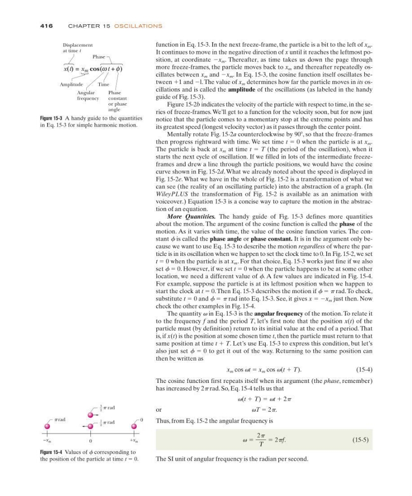
more freeze-frames, the particle moves back to x m and thereafter repeatedly oscillates between x m and Ϫx m . In Eq. 15-3, the cosine function itself oscillates between ϩ1 and Ϫl. The value of x m determines how far the particle moves in its oscillations and is called the amplitude of the oscillations (as labeled in the handy
guide of Fig. 15-3).
Figure 15-2b indicates the velocity of the particle with respect to time, in the series of freeze-frames. We’ll get to a function for the velocity soon, but for now just
notice that the particle comes to a momentary stop at the extreme points and has
its greatest speed (longest velocity vector) as it passes through the center point.
Mentally rotate Fig. 15-2a counterclockwise by 90Њ, so that the freeze-frames
then progress rightward with time. We set time t ϭ 0 when the particle is at x m .
The particle is back at x m at time t ϭ T (the period of the oscillation), when it
starts the next cycle of oscillation. If we filled in lots of the intermediate freezeframes and drew a line through the particle positions, we would have the cosine
curve shown in Fig. 15-2d. What we already noted about the speed is displayed in
Fig. 15-2e. What we have in the whole of Fig. 15-2 is a transformation of what we
can see (the reality of an oscillating particle) into the abstraction of a graph. (In
WileyPLUS the transformation of Fig. 15-2 is available as an animation with
voiceover.) Equation 15-3 is a concise way to capture the motion in the abstraction of an equation.
More Quantities. The handy guide of Fig. 15-3 defines more quantities
about the motion. The argument of the cosine function is called the phase of the
motion. As it varies with time, the value of the cosine function varies. The constant f is called the phase angle or phase constant. It is in the argument only because we want to use Eq. 15-3 to describe the motion regardless of where the particle is in its oscillation when we happen to set the clock time to 0. In Fig. 15-2, we set
t ϭ 0 when the particle is at x m . For that choice, Eq. 15-3 works just fine if we also
set f ϭ 0. However, if we set t ϭ 0 when the particle happens to be at some other
location, we need a different value of f. A few values are indicated in Fig. 15-4.
For example, suppose the particle is at its leftmost position when we happen to
start the clock at t ϭ 0. Then Eq. 15-3 describes the motion if f ϭ p rad. To check,
substitute t ϭ 0 and f ϭ p rad into Eq. 15-3. See, it gives x ϭ Ϫx m just then. Now
check the other examples in Fig. 15-4.
The quantity v in Eq. 15-3 is the angular frequency of the motion. To relate it
to the frequency f and the period T, let’s first note that the position x(t) of the
particle must (by definition) return to its initial value at the end of a period. That
is, if x(t) is the position at some chosen time t, then the particle must return to that
same position at time t ϩ T. Let’s use Eq. 15-3 to express this condition, but let’s
also just set f ϭ 0 to get it out of the way. Returning to the same position can
then be written as
x m cos vt ϭ x m cos v(t ϩ T).
(15-4)
The cosine function first repeats itself when its argument (the phase, remember)
has increased by 2p rad. So, Eq. 15-4 tells us that
v(t ϩ T) ϭ vt ϩ 2p
or
vT ϭ 2p.
Thus, from Eq. 15-2 the angular frequency is
(15-5)
The SI unit of angular frequency is the radian per second.
v ϭ
2p
⌻
ϭ 2pf.
Figure 15-3 A handy guide to the quantities
in Eq. 15-3 for simple harmonic motion.
Displacement
at time t
Amplitude
Angular
frequency
Time
Phase
constant
or phase
angle
Phase
x(t) = x m cos( t + )
ω φ
0
+x m
–x m
0
p rad
p rad
3
2
1
2
p rad
Figure 15-4 Values of f corresponding to
the position of the particle at time t ϭ 0.
CHAPTE R 15 OSCI LL ATIONS
function in Eq. 15-3. In the next freeze-frame, the particle is a bit to the left of x m .
It continues to move in the negative direction of x until it reaches the leftmost position, at coordinate Ϫx m . Thereafter, as time takes us down the page through
more freeze-frames, the particle moves back to x m and thereafter repeatedly oscillates between x m and Ϫx m . In Eq. 15-3, the cosine function itself oscillates between ϩ1 and Ϫl. The value of x m determines how far the particle moves in its oscillations and is called the amplitude of the oscillations (as labeled in the handy
guide of Fig. 15-3).
Figure 15-2b indicates the velocity of the particle with respect to time, in the series of freeze-frames. We’ll get to a function for the velocity soon, but for now just
notice that the particle comes to a momentary stop at the extreme points and has
its greatest speed (longest velocity vector) as it passes through the center point.
Mentally rotate Fig. 15-2a counterclockwise by 90Њ, so that the freeze-frames
then progress rightward with time. We set time t ϭ 0 when the particle is at x m .
The particle is back at x m at time t ϭ T (the period of the oscillation), when it
starts the next cycle of oscillation. If we filled in lots of the intermediate freezeframes and drew a line through the particle positions, we would have the cosine
curve shown in Fig. 15-2d. What we already noted about the speed is displayed in
Fig. 15-2e. What we have in the whole of Fig. 15-2 is a transformation of what we
can see (the reality of an oscillating particle) into the abstraction of a graph. (In
WileyPLUS the transformation of Fig. 15-2 is available as an animation with
voiceover.) Equation 15-3 is a concise way to capture the motion in the abstraction of an equation.
More Quantities. The handy guide of Fig. 15-3 defines more quantities
about the motion. The argument of the cosine function is called the phase of the
motion. As it varies with time, the value of the cosine function varies. The constant f is called the phase angle or phase constant. It is in the argument only because we want to use Eq. 15-3 to describe the motion regardless of where the particle is in its oscillation when we happen to set the clock time to 0. In Fig. 15-2, we set
t ϭ 0 when the particle is at x m . For that choice, Eq. 15-3 works just fine if we also
set f ϭ 0. However, if we set t ϭ 0 when the particle happens to be at some other
location, we need a different value of f. A few values are indicated in Fig. 15-4.
For example, suppose the particle is at its leftmost position when we happen to
start the clock at t ϭ 0. Then Eq. 15-3 describes the motion if f ϭ p rad. To check,
substitute t ϭ 0 and f ϭ p rad into Eq. 15-3. See, it gives x ϭ Ϫx m just then. Now
check the other examples in Fig. 15-4.
The quantity v in Eq. 15-3 is the angular frequency of the motion. To relate it
to the frequency f and the period T, let’s first note that the position x(t) of the
particle must (by definition) return to its initial value at the end of a period. That
is, if x(t) is the position at some chosen time t, then the particle must return to that
same position at time t ϩ T. Let’s use Eq. 15-3 to express this condition, but let’s
also just set f ϭ 0 to get it out of the way. Returning to the same position can
then be written as
x m cos vt ϭ x m cos v(t ϩ T).
(15-4)
The cosine function first repeats itself when its argument (the phase, remember)
has increased by 2p rad. So, Eq. 15-4 tells us that
v(t ϩ T) ϭ vt ϩ 2p
or
vT ϭ 2p.
Thus, from Eq. 15-2 the angular frequency is
(15-5)
The SI unit of angular frequency is the radian per second.
v ϭ
2p
⌻
ϭ 2pf.
Figure 15-3 A handy guide to the quantities
in Eq. 15-3 for simple harmonic motion.
Displacement
at time t
Amplitude
Angular
frequency
Time
Phase
constant
or phase
angle
Phase
x(t) = x m cos( t + )
ω φ
0
+x m
–x m
0
p rad
p rad
3
2
1
2
p rad
Figure 15-4 Values of f corresponding to
the position of the particle at time t ϭ 0.