

want the average force F avg on the wall during the bombardment — that is, the average force during a large number of collisions.
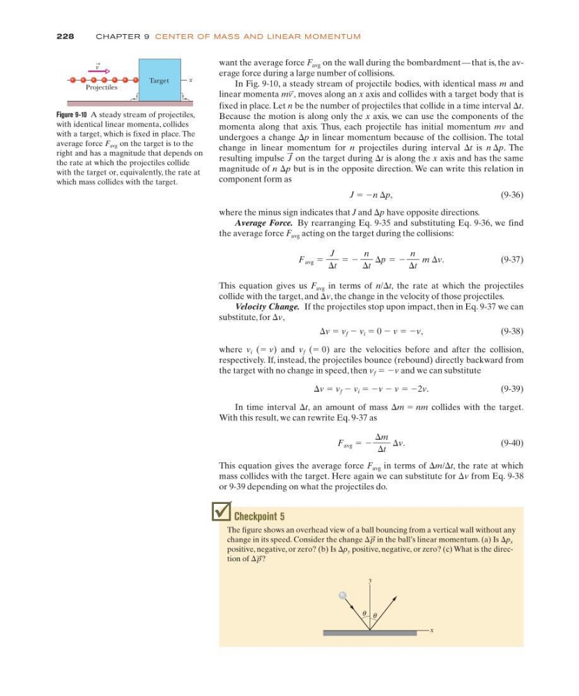
In Fig. 9-10, a steady stream of projectile bodies, with identical mass m and
linear momenta
moves along an x axis and collides with a target body that is
mv
:
,
228
CHAPTE R 9 CE NTE R OF MASS AN D LI N EAR M OM E NTU M
Figure 9-10 A steady stream of projectiles,
with identical linear momenta, collides
with a target, which is fixed in place. The
average force F avg on the target is to the
right and has a magnitude that depends on
the rate at which the projectiles collide
with the target or, equivalently, the rate at
which mass collides with the target.
x
Target
v
Projectiles
fixed in place. Let n be the number of projectiles that collide in a time interval ⌬t.
Because the motion is along only the x axis, we can use the components of the
momenta along that axis. Thus, each projectile has initial momentum mv and
undergoes a change ⌬p in linear momentum because of the collision. The total
change in linear momentum for n projectiles during interval ⌬t is n ⌬p. The
resulting impulse on the target during ⌬t is along the x axis and has the same
magnitude of n ⌬p but is in the opposite direction. We can write this relation in
component form as
J ϭ Ϫn ⌬p,
( 9 - 3 6 )
where the minus sign indicates that J and ⌬p have opposite directions.
Average Force. By rearranging Eq. 9-35 and substituting Eq. 9-36, we find
the average force F avg acting on the target during the collisions:
(9-37)
This equation gives us F avg in terms of n/⌬t, the rate at which the projectiles
collide with the target, and ⌬v, the change in the velocity of those projectiles.
Velocity Change. If the projectiles stop upon impact, then in Eq. 9-37 we can
substitute, for ⌬v,
⌬v ϭ v f Ϫ v i ϭ 0 Ϫ v ϭ Ϫv,
( 9 - 3 8 )
where v i (ϭ v) and v f (ϭ 0) are the velocities before and after the collision,
respectively. If, instead, the projectiles bounce (rebound) directly backward from
the target with no change in speed, then v f ϭ Ϫv and we can substitute
⌬v ϭ v f Ϫ v i ϭ Ϫv Ϫ v ϭ Ϫ2v.
( 9 - 3 9 )
In time interval ⌬t, an amount of mass ⌬m ϭ nm collides with the target.
With this result, we can rewrite Eq. 9-37 as
(9-40)
This equation gives the average force F avg in terms of ⌬m/⌬t, the rate at which
mass collides with the target. Here again we can substitute for ⌬v from Eq. 9-38
or 9-39 depending on what the projectiles do.
F avg ϭ Ϫ
⌬m
⌬t
⌬v.
F avg ϭ
J
⌬t
ϭ Ϫ
n
⌬t
⌬p ϭ Ϫ
n
⌬t
m ⌬v.
J
:
Checkpoint 5
The figure shows an overhead view of a ball bouncing from a vertical wall without any
change in its speed. Consider the change
in the ball’s linear momentum. (a) Is ⌬p x
positive, negative, or zero? (b) Is ⌬p y positive, negative, or zero? (c) What is the direction of
?
⌬p
:
⌬p
:
θ
θ
y
x
In Fig. 9-10, a steady stream of projectile bodies, with identical mass m and
linear momenta
moves along an x axis and collides with a target body that is
mv
:
,
228
CHAPTE R 9 CE NTE R OF MASS AN D LI N EAR M OM E NTU M
Figure 9-10 A steady stream of projectiles,
with identical linear momenta, collides
with a target, which is fixed in place. The
average force F avg on the target is to the
right and has a magnitude that depends on
the rate at which the projectiles collide
with the target or, equivalently, the rate at
which mass collides with the target.
x
Target
v
Projectiles
fixed in place. Let n be the number of projectiles that collide in a time interval ⌬t.
Because the motion is along only the x axis, we can use the components of the
momenta along that axis. Thus, each projectile has initial momentum mv and
undergoes a change ⌬p in linear momentum because of the collision. The total
change in linear momentum for n projectiles during interval ⌬t is n ⌬p. The
resulting impulse on the target during ⌬t is along the x axis and has the same
magnitude of n ⌬p but is in the opposite direction. We can write this relation in
component form as
J ϭ Ϫn ⌬p,
( 9 - 3 6 )
where the minus sign indicates that J and ⌬p have opposite directions.
Average Force. By rearranging Eq. 9-35 and substituting Eq. 9-36, we find
the average force F avg acting on the target during the collisions:
(9-37)
This equation gives us F avg in terms of n/⌬t, the rate at which the projectiles
collide with the target, and ⌬v, the change in the velocity of those projectiles.
Velocity Change. If the projectiles stop upon impact, then in Eq. 9-37 we can
substitute, for ⌬v,
⌬v ϭ v f Ϫ v i ϭ 0 Ϫ v ϭ Ϫv,
( 9 - 3 8 )
where v i (ϭ v) and v f (ϭ 0) are the velocities before and after the collision,
respectively. If, instead, the projectiles bounce (rebound) directly backward from
the target with no change in speed, then v f ϭ Ϫv and we can substitute
⌬v ϭ v f Ϫ v i ϭ Ϫv Ϫ v ϭ Ϫ2v.
( 9 - 3 9 )
In time interval ⌬t, an amount of mass ⌬m ϭ nm collides with the target.
With this result, we can rewrite Eq. 9-37 as
(9-40)
This equation gives the average force F avg in terms of ⌬m/⌬t, the rate at which
mass collides with the target. Here again we can substitute for ⌬v from Eq. 9-38
or 9-39 depending on what the projectiles do.
F avg ϭ Ϫ
⌬m
⌬t
⌬v.
F avg ϭ
J
⌬t
ϭ Ϫ
n
⌬t
⌬p ϭ Ϫ
n
⌬t
m ⌬v.
J
:
Checkpoint 5
The figure shows an overhead view of a ball bouncing from a vertical wall without any
change in its speed. Consider the change
in the ball’s linear momentum. (a) Is ⌬p x
positive, negative, or zero? (b) Is ⌬p y positive, negative, or zero? (c) What is the direction of
?
⌬p
:
⌬p
:
θ
θ
y
x