

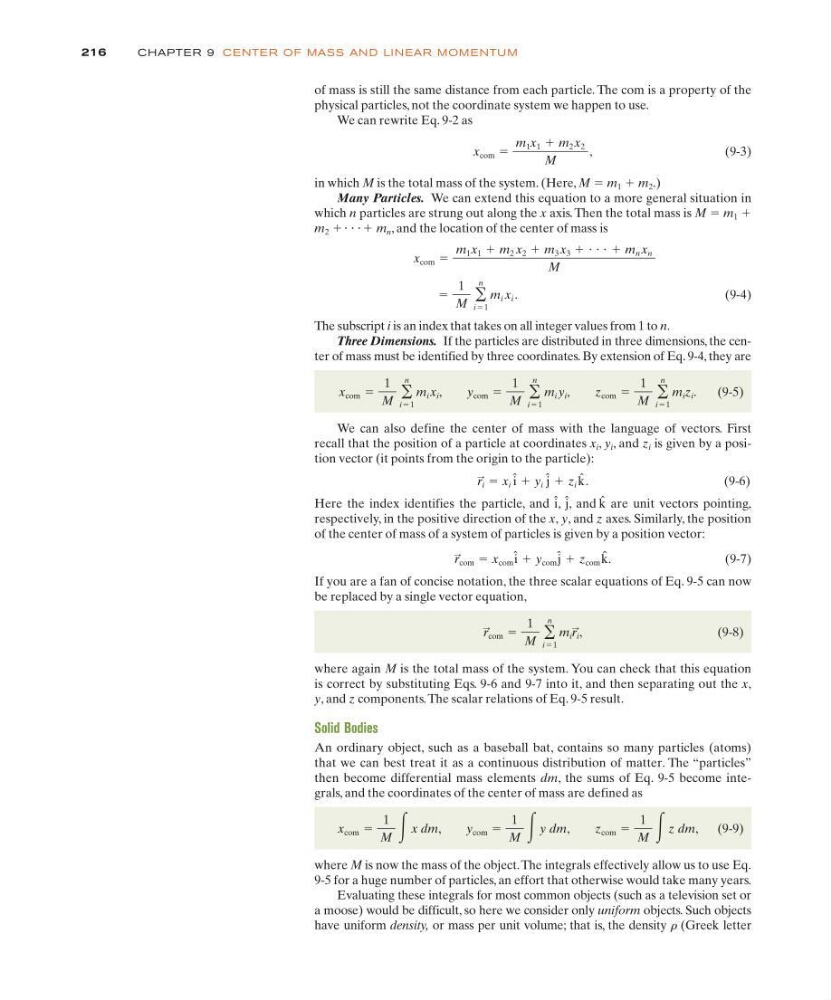
of mass is still the same distance from each particle. The com is a property of the
physical particles, not the coordinate system we happen to use.
We can rewrite Eq. 9-2 as
(9-3)
in which M is the total mass of the system. (Here, M ϭ m 1 ϩ m 2 .)
Many Particles. We can extend this equation to a more general situation in
which n particles are strung out along the x axis. Then the total mass is M ϭ m 1 ϩ
m 2 ϩ
ϩm n , and the location of the center of mass is
(9-4)
The subscript i is an index that takes on all integer values from 1 to n.
Three Dimensions. If the particles are distributed in three dimensions, the center of mass must be identified by three coordinates. By extension of Eq. 9-4, they are
(9-5)
We can also define the center of mass with the language of vectors. First
recall that the position of a particle at coordinates x i , y i , and z i is given by a position vector (it points from the origin to the particle):
(9-6)
Here the index identifies the particle, and i
ˆ , ˆ j, and ˆ
k are unit vectors pointing,
respectively, in the positive direction of the x, y, and z axes. Similarly, the position
of the center of mass of a system of particles is given by a position vector:
(9-7)
If you are a fan of concise notation, the three scalar equations of Eq. 9-5 can now
be replaced by a single vector equation,
(9-8)
where again M is the total mass of the system. You can check that this equation
is correct by substituting Eqs. 9-6 and 9-7 into it, and then separating out the x,
y, and z components. The scalar relations of Eq. 9-5 result.
Solid Bodies
An ordinary object, such as a baseball bat, contains so many particles (atoms)
that we can best treat it as a continuous distribution of matter. The “particles”
then become differential mass elements dm, the sums of Eq. 9-5 become integrals, and the coordinates of the center of mass are defined as
(9-9)
where M is now the mass of the object.The integrals effectively allow us to use Eq.
9-5 for a huge number of particles, an effort that otherwise would take many years.
Evaluating these integrals for most common objects (such as a television set or
a moose) would be difficult, so here we consider only uniform objects. Such objects
have uniform density, or mass per unit volume; that is, the density r (Greek letter
x com ϭ
1
M
͵xdm, y com ϭ
1
M
͵ydm, z com ϭ
1
M
͵zdm,
r com
:
ϭ
1
M ͚
n
iϭ1
m i r i
:
,
r com
:
ϭ x com ˆ i ϩ y com ˆ j ϩ z com ˆ
k.
r i
: ϭ x i i ˆ ϩ y i j
ˆ ϩ z i k ˆ .
x com ϭ
1
M ͚
n
iϭ1
m i x i ,
y com ϭ
1
M ͚
n
iϭ1
m i y i ,
z com ϭ
1
M ͚
n
iϭ1
m i z i .
ϭ
1
M ͚
n
iϭ1
m i x i .
x com ϭ
m 1 x 1 ϩ m 2 x 2 ϩ m 3 x 3 ϩ и и и ϩ m n x n
M
и и и
x com ϭ
m 1 x 1 ϩ m 2 x 2
M
,
216
CHAPTE R 9 CE NTE R OF MASS AN D LI N EAR M OM E NTU M
physical particles, not the coordinate system we happen to use.
We can rewrite Eq. 9-2 as
(9-3)
in which M is the total mass of the system. (Here, M ϭ m 1 ϩ m 2 .)
Many Particles. We can extend this equation to a more general situation in
which n particles are strung out along the x axis. Then the total mass is M ϭ m 1 ϩ
m 2 ϩ
ϩm n , and the location of the center of mass is
(9-4)
The subscript i is an index that takes on all integer values from 1 to n.
Three Dimensions. If the particles are distributed in three dimensions, the center of mass must be identified by three coordinates. By extension of Eq. 9-4, they are
(9-5)
We can also define the center of mass with the language of vectors. First
recall that the position of a particle at coordinates x i , y i , and z i is given by a position vector (it points from the origin to the particle):
(9-6)
Here the index identifies the particle, and i
ˆ , ˆ j, and ˆ
k are unit vectors pointing,
respectively, in the positive direction of the x, y, and z axes. Similarly, the position
of the center of mass of a system of particles is given by a position vector:
(9-7)
If you are a fan of concise notation, the three scalar equations of Eq. 9-5 can now
be replaced by a single vector equation,
(9-8)
where again M is the total mass of the system. You can check that this equation
is correct by substituting Eqs. 9-6 and 9-7 into it, and then separating out the x,
y, and z components. The scalar relations of Eq. 9-5 result.
Solid Bodies
An ordinary object, such as a baseball bat, contains so many particles (atoms)
that we can best treat it as a continuous distribution of matter. The “particles”
then become differential mass elements dm, the sums of Eq. 9-5 become integrals, and the coordinates of the center of mass are defined as
(9-9)
where M is now the mass of the object.The integrals effectively allow us to use Eq.
9-5 for a huge number of particles, an effort that otherwise would take many years.
Evaluating these integrals for most common objects (such as a television set or
a moose) would be difficult, so here we consider only uniform objects. Such objects
have uniform density, or mass per unit volume; that is, the density r (Greek letter
x com ϭ
1
M
͵xdm, y com ϭ
1
M
͵ydm, z com ϭ
1
M
͵zdm,
r com
:
ϭ
1
M ͚
n
iϭ1
m i r i
:
,
r com
:
ϭ x com ˆ i ϩ y com ˆ j ϩ z com ˆ
k.
r i
: ϭ x i i ˆ ϩ y i j
ˆ ϩ z i k ˆ .
x com ϭ
1
M ͚
n
iϭ1
m i x i ,
y com ϭ
1
M ͚
n
iϭ1
m i y i ,
z com ϭ
1
M ͚
n
iϭ1
m i z i .
ϭ
1
M ͚
n
iϭ1
m i x i .
x com ϭ
m 1 x 1 ϩ m 2 x 2 ϩ m 3 x 3 ϩ и и и ϩ m n x n
M
и и и
x com ϭ
m 1 x 1 ϩ m 2 x 2
M
,
216
CHAPTE R 9 CE NTE R OF MASS AN D LI N EAR M OM E NTU M