

go the other way; that is, we know the potential energy function U(x) and want
to find the force.
For one-dimensional motion, the work W done by a force that acts on a particle as the particle moves through a distance ⌬x is F(x) ⌬x. We can then write
Eq. 8-1 as
⌬U(x) ϭ ϪW ϭ ϪF(x) ⌬x.
( 8 - 2 1 )
Solving for F(x) and passing to the differential limit yield
(one-dimensional motion),
(8-22)
which is the relation we sought.
We can check this result by putting
, which is the elastic potential energy function for a spring force. Equation 8-22 then yields, as expected,
F(x) ϭ Ϫkx, which is Hooke’s law. Similarly, we can substitute U(x) ϭ mgx,
which is the gravitational potential energy function for a particle – Earth system,
with a particle of mass m at height x above Earth’s surface. Equation 8-22 then
yields F ϭ Ϫmg, which is the gravitational force on the particle.
The Potential Energy Curve
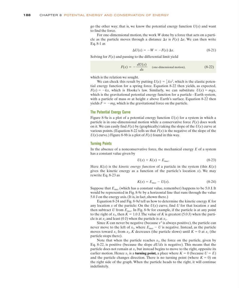
Figure 8-9a is a plot of a potential energy function U(x) for a system in which a
particle is in one-dimensional motion while a conservative force F(x) does work
on it. We can easily find F(x) by (graphically) taking the slope of the U(x) curve at
various points. (Equation 8-22 tells us that F(x) is the negative of the slope of the
U(x) curve.) Figure 8-9b is a plot of F(x) found in this way.
Turning Points
In the absence of a nonconservative force, the mechanical energy E of a system
has a constant value given by
U(x) ϩ K(x) ϭ E mec .
( 8 - 2 3 )
Here K(x) is the kinetic energy function of a particle in the system (this K(x)
gives the kinetic energy as a function of the particle’s location x). We may
rewrite Eq. 8-23 as
K(x) ϭ E mec Ϫ U(x).
(8-24)
Suppose that E mec (which has a constant value, remember) happens to be 5.0 J. It
would be represented in Fig. 8-9c by a horizontal line that runs through the value
5.0 J on the energy axis. (It is, in fact, shown there.)
Equation 8-24 and Fig. 8-9d tell us how to determine the kinetic energy K for
any location x of the particle: On the U(x) curve, find U for that location x and
then subtract U from E mec . In Fig. 8-9e for example, if the particle is at any point
to the right of x 5 , then K ϭ 1.0 J. The value of K is greatest (5.0 J) when the particle is at x 2 and least (0 J) when the particle is at x 1 .
Since K can never be negative (because v
2
is always positive), the particle can
never move to the left of x 1 , where E mec Ϫ U is negative. Instead, as the particle
moves toward x 1 from x 2 , K decreases (the particle slows) until K ϭ 0 at x 1 (the
particle stops there).
Note that when the particle reaches x 1 , the force on the particle, given by
Eq. 8-22, is positive (because the slope dU/dx is negative). This means that the
particle does not remain at x 1 but instead begins to move to the right, opposite its
earlier motion. Hence x 1 is a turning point, a place where K ϭ 0 (because U ϭ E)
and the particle changes direction. There is no turning point (where K ϭ 0) on
the right side of the graph. When the particle heads to the right, it will continue
indefinitely.
U(x) ϭ
1
2 kx
2
F(x) ϭ Ϫ
dU(x)
dx
188
CHAPTE R 8 POTE NTIAL E N E RGY AN D CONSE RVATION OF ENERGY
to find the force.
For one-dimensional motion, the work W done by a force that acts on a particle as the particle moves through a distance ⌬x is F(x) ⌬x. We can then write
Eq. 8-1 as
⌬U(x) ϭ ϪW ϭ ϪF(x) ⌬x.
( 8 - 2 1 )
Solving for F(x) and passing to the differential limit yield
(one-dimensional motion),
(8-22)
which is the relation we sought.
We can check this result by putting
, which is the elastic potential energy function for a spring force. Equation 8-22 then yields, as expected,
F(x) ϭ Ϫkx, which is Hooke’s law. Similarly, we can substitute U(x) ϭ mgx,
which is the gravitational potential energy function for a particle – Earth system,
with a particle of mass m at height x above Earth’s surface. Equation 8-22 then
yields F ϭ Ϫmg, which is the gravitational force on the particle.
The Potential Energy Curve
Figure 8-9a is a plot of a potential energy function U(x) for a system in which a
particle is in one-dimensional motion while a conservative force F(x) does work
on it. We can easily find F(x) by (graphically) taking the slope of the U(x) curve at
various points. (Equation 8-22 tells us that F(x) is the negative of the slope of the
U(x) curve.) Figure 8-9b is a plot of F(x) found in this way.
Turning Points
In the absence of a nonconservative force, the mechanical energy E of a system
has a constant value given by
U(x) ϩ K(x) ϭ E mec .
( 8 - 2 3 )
Here K(x) is the kinetic energy function of a particle in the system (this K(x)
gives the kinetic energy as a function of the particle’s location x). We may
rewrite Eq. 8-23 as
K(x) ϭ E mec Ϫ U(x).
(8-24)
Suppose that E mec (which has a constant value, remember) happens to be 5.0 J. It
would be represented in Fig. 8-9c by a horizontal line that runs through the value
5.0 J on the energy axis. (It is, in fact, shown there.)
Equation 8-24 and Fig. 8-9d tell us how to determine the kinetic energy K for
any location x of the particle: On the U(x) curve, find U for that location x and
then subtract U from E mec . In Fig. 8-9e for example, if the particle is at any point
to the right of x 5 , then K ϭ 1.0 J. The value of K is greatest (5.0 J) when the particle is at x 2 and least (0 J) when the particle is at x 1 .
Since K can never be negative (because v
2
is always positive), the particle can
never move to the left of x 1 , where E mec Ϫ U is negative. Instead, as the particle
moves toward x 1 from x 2 , K decreases (the particle slows) until K ϭ 0 at x 1 (the
particle stops there).
Note that when the particle reaches x 1 , the force on the particle, given by
Eq. 8-22, is positive (because the slope dU/dx is negative). This means that the
particle does not remain at x 1 but instead begins to move to the right, opposite its
earlier motion. Hence x 1 is a turning point, a place where K ϭ 0 (because U ϭ E)
and the particle changes direction. There is no turning point (where K ϭ 0) on
the right side of the graph. When the particle heads to the right, it will continue
indefinitely.
U(x) ϭ
1
2 kx
2
F(x) ϭ Ϫ
dU(x)
dx
188
CHAPTE R 8 POTE NTIAL E N E RGY AN D CONSE RVATION OF ENERGY