

81
REVIEW & SUM MARY
velocity of plane
velocity of plane
velocity of wind
relative to ground
ϭ relative to wind
ϩ relative to ground.
(PG)
( PW)
( WG)
This relation is written in vector notation as
(4-46)
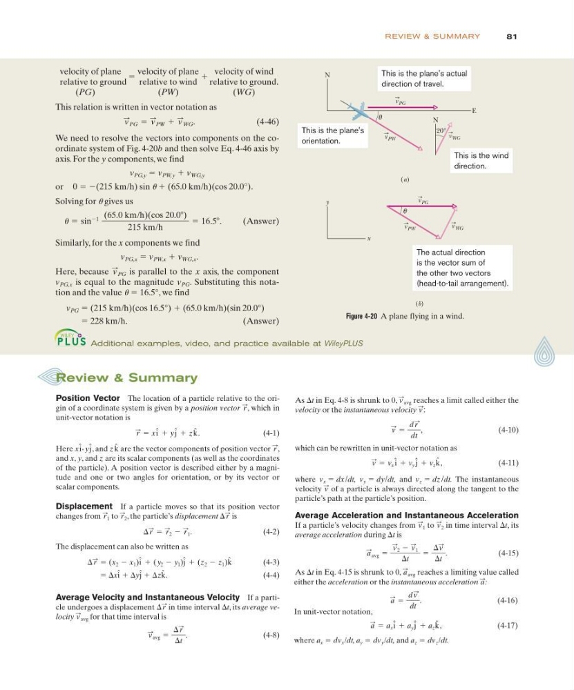
We need to resolve the vectors into components on the coordinate system of Fig. 4-20b and then solve Eq. 4-46 axis by
axis. For the y components, we find
v PG,y ϭ v PW,y ϩ v WG,y
or 0 ϭ Ϫ(215 km/h) sin u ϩ (65.0 km/h)(cos 20.0°).
Solving for u gives us
(Answer)
Similarly, for the x components we find
v PG,x ϭ v PW,x ϩ v WG,x .
Here, because
is parallel to the x axis, the component
v PG,x is equal to the magnitude v PG . Substituting this notation and the value u ϭ 16.5°, we find
v PG ϭ (215 km/h)(cos 16.5°) ϩ (65.0 km/h)(sin 20.0°)
ϭ 228 km/h.
(Answer)
v
:
PG
ϭ sin
Ϫ1
(65.0 km/h)(cos 20.0Њ)
215 km/h
ϭ 16.5Њ.
v
:
PG ϭ v
:
PW ϩ v
:
WG .
θ
θ
v PG
v PW
v WG
v PG
v PW
v WG
N
y
N
E
20°
x
(a)
(b)
This is the plane's actual
direction of travel.
This is the wind
direction.
The actual direction
is the vector sum of
the other two vectors
(head-to-tail arrangement).
This is the plane's
orientation.
Figure 4-20 A plane flying in a wind.
Additional examples, video, and practice available at WileyPLUS
Review & Summary
Position Vector The location of a particle relative to the origin of a coordinate system is given by a position vector , which in
unit-vector notation is
(4-1)
Here x , y , and z are the vector components of position vector ,
and x, y, and z are its scalar components (as well as the coordinates
of the particle). A position vector is described either by a magnitude and one or two angles for orientation, or by its vector or
scalar components.
Displacement If a particle moves so that its position vector
changes from to , the particle’s displacement
is
(4-2)
The displacement can also be written as
(4-3)
ϭ ⌬x ϩ ⌬y ϩ ⌬z .
( 4 - 4 )
Average Velocity and Instantaneous Velocity If a particle undergoes a displacement
in time interval ⌬t, its average velocity
for that time interval is
(4-8)
v
:
avg ϭ
⌬ r
:
⌬t
.
v
:
avg
⌬ r
:
k ˆ
j
ˆ
i
ˆ
⌬ r
: ϭ (x 2 Ϫ x 1 )i ˆ ϩ ( y 2 Ϫ y 1 )j ˆ ϩ (z 2 Ϫ z 1 )k ˆ
⌬ r
: ϭ r
:
2 Ϫ r
:
1 .
⌬ r
:
r
:
2
r
:
1
r
:
k ˆ
j
ˆ
i
ˆ
r
: ϭ xi ˆ ϩ yj ˆ ϩ zk ˆ .
r
:
As ⌬t in Eq. 4-8 is shrunk to 0,
reaches a limit called either the
velocity or the instantaneous velocity :
(4-10)
which can be rewritten in unit-vector notation as
(4-11)
where v x ϭ dx/dt, v y ϭ dy/dt, and v z ϭ dz/dt. The instantaneous
velocity of a particle is always directed along the tangent to the
particle’s path at the particle’s position.
Average Acceleration and Instantaneous Acceleration
If a particle’s velocity changes from to in time interval ⌬t, its
average acceleration during ⌬t is
(4-15)
As ⌬t in Eq. 4-15 is shrunk to 0,
reaches a limiting value called
a
:
avg
a
:
avg ϭ
v
:
2 Ϫ v
:
1
⌬t
ϭ
⌬v
:
⌬t
.
v
:
2
v
:
1
v
:
v
: ϭ v x i
ˆ ϩ v y j
ˆ ϩ v z k ˆ ,
v
: ϭ
d r
:
dt
,
v
:
v
:
avg
either the acceleration or the instantaneous acceleration :
(4-16)
In unit-vector notation,
(4-17)
where a x ϭ dv x /dt, a y ϭ dv y /dt, and a z ϭ dv z /dt.
a
: ϭ a x i ˆ ϩ a y j ˆ ϩ a z k ˆ ,
a
: ϭ
d v
:
dt
.
a
:
REVIEW & SUM MARY
velocity of plane
velocity of plane
velocity of wind
relative to ground
ϭ relative to wind
ϩ relative to ground.
(PG)
( PW)
( WG)
This relation is written in vector notation as
(4-46)
We need to resolve the vectors into components on the coordinate system of Fig. 4-20b and then solve Eq. 4-46 axis by
axis. For the y components, we find
v PG,y ϭ v PW,y ϩ v WG,y
or 0 ϭ Ϫ(215 km/h) sin u ϩ (65.0 km/h)(cos 20.0°).
Solving for u gives us
(Answer)
Similarly, for the x components we find
v PG,x ϭ v PW,x ϩ v WG,x .
Here, because
is parallel to the x axis, the component
v PG,x is equal to the magnitude v PG . Substituting this notation and the value u ϭ 16.5°, we find
v PG ϭ (215 km/h)(cos 16.5°) ϩ (65.0 km/h)(sin 20.0°)
ϭ 228 km/h.
(Answer)
v
:
PG
ϭ sin
Ϫ1
(65.0 km/h)(cos 20.0Њ)
215 km/h
ϭ 16.5Њ.
v
:
PG ϭ v
:
PW ϩ v
:
WG .
θ
θ
v PG
v PW
v WG
v PG
v PW
v WG
N
y
N
E
20°
x
(a)
(b)
This is the plane's actual
direction of travel.
This is the wind
direction.
The actual direction
is the vector sum of
the other two vectors
(head-to-tail arrangement).
This is the plane's
orientation.
Figure 4-20 A plane flying in a wind.
Additional examples, video, and practice available at WileyPLUS
Review & Summary
Position Vector The location of a particle relative to the origin of a coordinate system is given by a position vector , which in
unit-vector notation is
(4-1)
Here x , y , and z are the vector components of position vector ,
and x, y, and z are its scalar components (as well as the coordinates
of the particle). A position vector is described either by a magnitude and one or two angles for orientation, or by its vector or
scalar components.
Displacement If a particle moves so that its position vector
changes from to , the particle’s displacement
is
(4-2)
The displacement can also be written as
(4-3)
ϭ ⌬x ϩ ⌬y ϩ ⌬z .
( 4 - 4 )
Average Velocity and Instantaneous Velocity If a particle undergoes a displacement
in time interval ⌬t, its average velocity
for that time interval is
(4-8)
v
:
avg ϭ
⌬ r
:
⌬t
.
v
:
avg
⌬ r
:
k ˆ
j
ˆ
i
ˆ
⌬ r
: ϭ (x 2 Ϫ x 1 )i ˆ ϩ ( y 2 Ϫ y 1 )j ˆ ϩ (z 2 Ϫ z 1 )k ˆ
⌬ r
: ϭ r
:
2 Ϫ r
:
1 .
⌬ r
:
r
:
2
r
:
1
r
:
k ˆ
j
ˆ
i
ˆ
r
: ϭ xi ˆ ϩ yj ˆ ϩ zk ˆ .
r
:
As ⌬t in Eq. 4-8 is shrunk to 0,
reaches a limit called either the
velocity or the instantaneous velocity :
(4-10)
which can be rewritten in unit-vector notation as
(4-11)
where v x ϭ dx/dt, v y ϭ dy/dt, and v z ϭ dz/dt. The instantaneous
velocity of a particle is always directed along the tangent to the
particle’s path at the particle’s position.
Average Acceleration and Instantaneous Acceleration
If a particle’s velocity changes from to in time interval ⌬t, its
average acceleration during ⌬t is
(4-15)
As ⌬t in Eq. 4-15 is shrunk to 0,
reaches a limiting value called
a
:
avg
a
:
avg ϭ
v
:
2 Ϫ v
:
1
⌬t
ϭ
⌬v
:
⌬t
.
v
:
2
v
:
1
v
:
v
: ϭ v x i
ˆ ϩ v y j
ˆ ϩ v z k ˆ ,
v
: ϭ
d r
:
dt
,
v
:
v
:
avg
either the acceleration or the instantaneous acceleration :
(4-16)
In unit-vector notation,
(4-17)
where a x ϭ dv x /dt, a y ϭ dv y /dt, and a z ϭ dv z /dt.
a
: ϭ a x i ˆ ϩ a y j ˆ ϩ a z k ˆ ,
a
: ϭ
d v
:
dt
.
a
: