

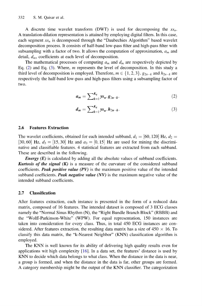
A discrete time wavelet transform (DWT) is used for decomposing the xs n .
A translation-dilation representation is attained by employing digital filters. In this case,
each segment xs n is decomposed through the “Daubechies Algorithm” based wavelet
decomposition process. It consists of half-band low-pass filter and high-pass filter with
subsampling with a factor of two. It allows the computation of approximation, a m and
detail, d m , coefficients at each level of decomposition.
The mathematical processes of computing a m and d m are respectively depicted by
Eq. (2) and Eq. (3). Where, m represents the level of decomposition. In this study a
third level of decomposition is employed. Therefore, m 2 1; 2; 3
f
g. g 2nÀk and h 2nÀk are
respectively the half-band low-pass and high-pass filters using a subsampling factor of
two.
a m ¼
X K g
k¼1
ys n : g 2nÀk :
ð2Þ
d m ¼
X K g
k¼1
ys n : h 2nÀk :
ð3Þ
2.6 Features Extraction
The wavelet coefficients, obtained for each intended subband, d 1 ¼ ½60; 120 Hz, d 2 ¼
½30; 60 Hz, d 3 ¼ ½15; 30 Hz and a 3 ¼ ½0; 15 Hz are used for mining the discriminative and classifiable features. 4 statistical features are extracted from each subband.
These are described in the following.
Energy (E) is calculated by adding all the absolute values of subband coefficients.
Kurtosis of the signal (K) is a measure of the curvature of the considered subband
coefficients. Peak positive value (PV) is the maximum positive value of the intended
subband coefficients. Peak negative value (NV) is the maximum negative value of the
intended subband coefficients.
2.7 Classification
After features extraction, each instance is presented in the form of a reduced data
matrix, composed of 16 features. The intended dataset is composed of 3 ECG classes
namely the “Normal Sinus Rhythm (N), the “Right Bundle Branch Block” (RBBB) and
the “Wolff-Parkinson-White” (WPW). For equal representation, 150 instances are
taken into consideration for every class. Thus, in total 450 ECG instances are considered. After features extraction, the resulting data matrix has a size of 450 Â 16. To
classify this data matrix, the “k-Nearest Neighbor” (KNN) classification algorithm is
employed.
The KNN is well known for its ability of delivering high quality results even for
applications wit high complexity [16]. In a data set, the features’ distance is used by
KNN to decide which data belongs to what class. When the distance in the data is near,
a group is formed, and when the distance in the data is far, other groups are formed.
A category membership might be the output of the KNN classifier. The categorization
332
S. M. Qaisar et al.
A translation-dilation representation is attained by employing digital filters. In this case,
each segment xs n is decomposed through the “Daubechies Algorithm” based wavelet
decomposition process. It consists of half-band low-pass filter and high-pass filter with
subsampling with a factor of two. It allows the computation of approximation, a m and
detail, d m , coefficients at each level of decomposition.
The mathematical processes of computing a m and d m are respectively depicted by
Eq. (2) and Eq. (3). Where, m represents the level of decomposition. In this study a
third level of decomposition is employed. Therefore, m 2 1; 2; 3
f
g. g 2nÀk and h 2nÀk are
respectively the half-band low-pass and high-pass filters using a subsampling factor of
two.
a m ¼
X K g
k¼1
ys n : g 2nÀk :
ð2Þ
d m ¼
X K g
k¼1
ys n : h 2nÀk :
ð3Þ
2.6 Features Extraction
The wavelet coefficients, obtained for each intended subband, d 1 ¼ ½60; 120 Hz, d 2 ¼
½30; 60 Hz, d 3 ¼ ½15; 30 Hz and a 3 ¼ ½0; 15 Hz are used for mining the discriminative and classifiable features. 4 statistical features are extracted from each subband.
These are described in the following.
Energy (E) is calculated by adding all the absolute values of subband coefficients.
Kurtosis of the signal (K) is a measure of the curvature of the considered subband
coefficients. Peak positive value (PV) is the maximum positive value of the intended
subband coefficients. Peak negative value (NV) is the maximum negative value of the
intended subband coefficients.
2.7 Classification
After features extraction, each instance is presented in the form of a reduced data
matrix, composed of 16 features. The intended dataset is composed of 3 ECG classes
namely the “Normal Sinus Rhythm (N), the “Right Bundle Branch Block” (RBBB) and
the “Wolff-Parkinson-White” (WPW). For equal representation, 150 instances are
taken into consideration for every class. Thus, in total 450 ECG instances are considered. After features extraction, the resulting data matrix has a size of 450 Â 16. To
classify this data matrix, the “k-Nearest Neighbor” (KNN) classification algorithm is
employed.
The KNN is well known for its ability of delivering high quality results even for
applications wit high complexity [16]. In a data set, the features’ distance is used by
KNN to decide which data belongs to what class. When the distance in the data is near,
a group is formed, and when the distance in the data is far, other groups are formed.
A category membership might be the output of the KNN classifier. The categorization
332
S. M. Qaisar et al.