

9.2 Finite Difference Methods
301
This equation is to be solved for u n+1 . If f is linear in u, it is a linear equation,
but if f is nonlinear in u, one needs approximate methods for nonlinear equations
(Chap. 7).
In our case, we have a system of linear ODEs (9.9)–(9.11). The Backward Euler
scheme applied to each equation leads to
u
n+1
0
− u
n
0
Δt
= s
(t n+1 ),
(9.16)
u
n+1
i
− u
n
i
Δt
=
β
Δx 2 (u
n+1
i+1 − 2u
n+1
i
+ u
n+1
i−1 ) + g i (t n+1 ),
(9.17)
i = 1, . . . , N − 1,
u
n+1
N − u
n
N
Δt
=
2β
Δx 2 (u
n+1
N−1 − u
n+1
N ) + g i (t n+1 ) .
(9.18)
This is a system of linear equations in the unknowns u
n+1
i
, i = 0, . . . , N, which is
easy to realize by writing out the equations for the case N = 3, collecting all the
unknown terms on the left-hand side and all the known terms on the right-hand side:
u
n+1
0
= u
n
0 + Δt s
(t n+1 ),
(9.19)
u
n+1
1
− Δt
β
Δx 2 (u
n+1
2
− 2u
n+1
1
+ u
n+1
0 ) = u
n
1 + Δt g 1 (t n+1 ),
(9.20)
u
n+1
2
− Δt
2β
Δx 2 (u
n+1
1
− u
n+1
2 ) = u
n
2 + Δt g 2 (t n+1 ) .
(9.21)
A system of linear equations like this, is usually written on matrix form Au = b,
where A is a coefficient matrix, u = (u
n+1
0 , . . . , n
n+1
N ) is the vector of unknowns,
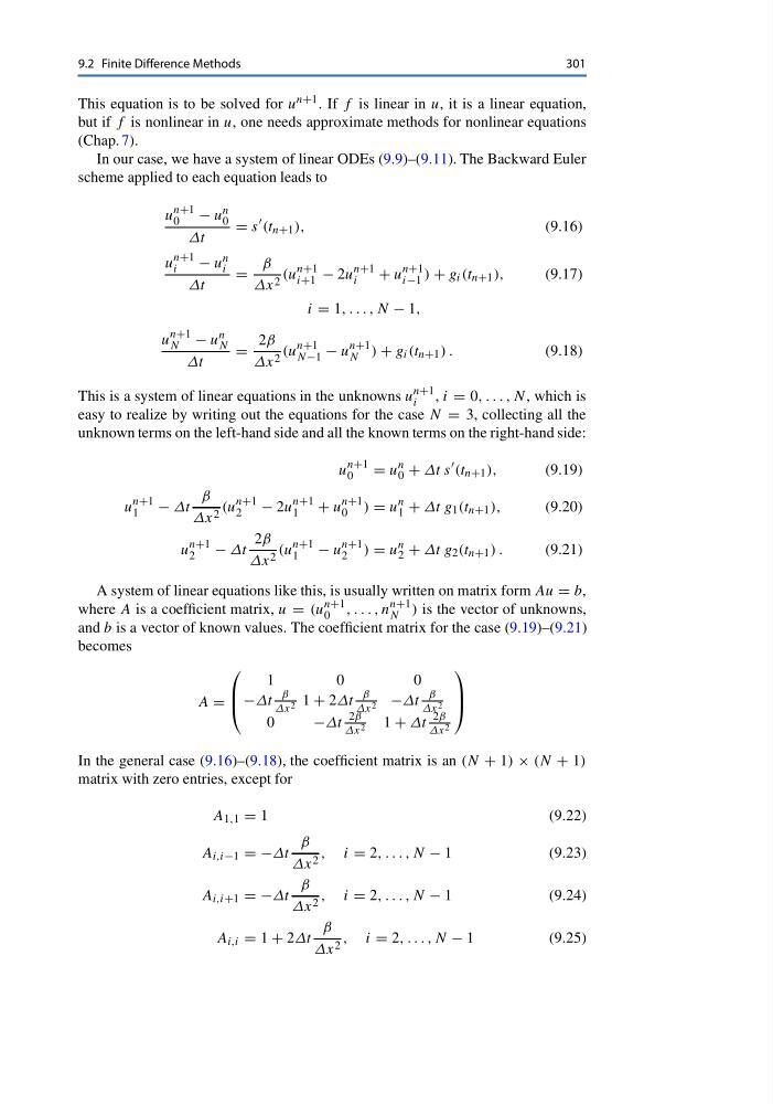
and b is a vector of known values. The coefficient matrix for the case (9.19)–(9.21)
becomes
A =
⎛
⎜
⎝
1
0
0
−Δt
β
Δx 2 1 + 2Δt
β
Δx 2 −Δt
β
Δx 2
0
−Δt
2β
Δx 2
1 + Δt
2β
Δx 2
⎞
⎟
⎠
In the general case (9.16)–(9.18), the coefficient matrix is an (N + 1) × (N + 1)
matrix with zero entries, except for
A 1,1 = 1
(9.22)
A i,i−1 = −Δt
β
Δx 2 , i = 2, . . . , N − 1
(9.23)
A i,i+1 = −Δt
β
Δx 2 , i = 2, . . . , N − 1
(9.24)
A i,i = 1 + 2Δt
β
Δx 2 , i = 2, . . . , N − 1
(9.25)
301
This equation is to be solved for u n+1 . If f is linear in u, it is a linear equation,
but if f is nonlinear in u, one needs approximate methods for nonlinear equations
(Chap. 7).
In our case, we have a system of linear ODEs (9.9)–(9.11). The Backward Euler
scheme applied to each equation leads to
u
n+1
0
− u
n
0
Δt
= s
(t n+1 ),
(9.16)
u
n+1
i
− u
n
i
Δt
=
β
Δx 2 (u
n+1
i+1 − 2u
n+1
i
+ u
n+1
i−1 ) + g i (t n+1 ),
(9.17)
i = 1, . . . , N − 1,
u
n+1
N − u
n
N
Δt
=
2β
Δx 2 (u
n+1
N−1 − u
n+1
N ) + g i (t n+1 ) .
(9.18)
This is a system of linear equations in the unknowns u
n+1
i
, i = 0, . . . , N, which is
easy to realize by writing out the equations for the case N = 3, collecting all the
unknown terms on the left-hand side and all the known terms on the right-hand side:
u
n+1
0
= u
n
0 + Δt s
(t n+1 ),
(9.19)
u
n+1
1
− Δt
β
Δx 2 (u
n+1
2
− 2u
n+1
1
+ u
n+1
0 ) = u
n
1 + Δt g 1 (t n+1 ),
(9.20)
u
n+1
2
− Δt
2β
Δx 2 (u
n+1
1
− u
n+1
2 ) = u
n
2 + Δt g 2 (t n+1 ) .
(9.21)
A system of linear equations like this, is usually written on matrix form Au = b,
where A is a coefficient matrix, u = (u
n+1
0 , . . . , n
n+1
N ) is the vector of unknowns,
and b is a vector of known values. The coefficient matrix for the case (9.19)–(9.21)
becomes
A =
⎛
⎜
⎝
1
0
0
−Δt
β
Δx 2 1 + 2Δt
β
Δx 2 −Δt
β
Δx 2
0
−Δt
2β
Δx 2
1 + Δt
2β
Δx 2
⎞
⎟
⎠
In the general case (9.16)–(9.18), the coefficient matrix is an (N + 1) × (N + 1)
matrix with zero entries, except for
A 1,1 = 1
(9.22)
A i,i−1 = −Δt
β
Δx 2 , i = 2, . . . , N − 1
(9.23)
A i,i+1 = −Δt
β
Δx 2 , i = 2, . . . , N − 1
(9.24)
A i,i = 1 + 2Δt
β
Δx 2 , i = 2, . . . , N − 1
(9.25)