

300
9 Solving Partial Differential Equations
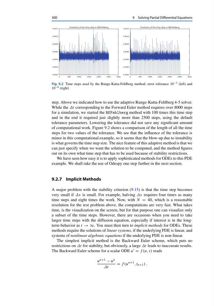
Fig. 9.2 Time steps used by the Runge-Kutta-Fehlberg method: error tolerance 10 −3 (left) and
10 −6 (right)
step. Above we indicated how to use the adaptive Runge-Kutta-Fehlberg 4-5 solver.
While the Δt corresponding to the Forward Euler method requires over 8000 steps
for a simulation, we started the RKFehlberg method with 100 times this time step
and in the end it required just slightly more than 2500 steps, using the default
tolerance parameters. Lowering the tolerance did not save any significant amount
of computational work. Figure 9.2 shows a comparison of the length of all the time
steps for two values of the tolerance. We see that the influence of the tolerance is
minor in this computational example, so it seems that the blow-up due to instability
is what governs the time step size. The nice feature of this adaptive method is that we
can just specify when we want the solution to be computed, and the method figures
out on its own what time step that has to be used because of stability restrictions.
We have seen how easy it is to apply sophisticated methods for ODEs to this PDE
example. We shall take the use of Odespy one step further in the next section.
9.2.7 Implicit Methods
A major problem with the stability criterion (9.15) is that the time step becomes
very small if Δx is small. For example, halving Δx requires four times as many
time steps and eight times the work. Now, with N = 40, which is a reasonable
resolution for the test problem above, the computations are very fast. What takes
time, is the visualization on the screen, but for that purpose one can visualize only
a subset of the time steps. However, there are occasions when you need to take
larger time steps with the diffusion equation, especially if interest is in the longterm behavior as t → ∞. You must then turn to implicit methods for ODEs. These
methods require the solutions of linear systems, if the underlying PDE is linear, and
systems of nonlinear algebraic equations if the underlying PDE is non-linear.
The simplest implicit method is the Backward Euler scheme, which puts no
restrictions on Δt for stability, but obviously, a large Δt leads to inaccurate results.
The Backward Euler scheme for a scalar ODE u = f (u, t) reads
u n+1 − u n
Δt
= f (u
n+1 , t n+1 ) .
9 Solving Partial Differential Equations
Fig. 9.2 Time steps used by the Runge-Kutta-Fehlberg method: error tolerance 10 −3 (left) and
10 −6 (right)
step. Above we indicated how to use the adaptive Runge-Kutta-Fehlberg 4-5 solver.
While the Δt corresponding to the Forward Euler method requires over 8000 steps
for a simulation, we started the RKFehlberg method with 100 times this time step
and in the end it required just slightly more than 2500 steps, using the default
tolerance parameters. Lowering the tolerance did not save any significant amount
of computational work. Figure 9.2 shows a comparison of the length of all the time
steps for two values of the tolerance. We see that the influence of the tolerance is
minor in this computational example, so it seems that the blow-up due to instability
is what governs the time step size. The nice feature of this adaptive method is that we
can just specify when we want the solution to be computed, and the method figures
out on its own what time step that has to be used because of stability restrictions.
We have seen how easy it is to apply sophisticated methods for ODEs to this PDE
example. We shall take the use of Odespy one step further in the next section.
9.2.7 Implicit Methods
A major problem with the stability criterion (9.15) is that the time step becomes
very small if Δx is small. For example, halving Δx requires four times as many
time steps and eight times the work. Now, with N = 40, which is a reasonable
resolution for the test problem above, the computations are very fast. What takes
time, is the visualization on the screen, but for that purpose one can visualize only
a subset of the time steps. However, there are occasions when you need to take
larger time steps with the diffusion equation, especially if interest is in the longterm behavior as t → ∞. You must then turn to implicit methods for ODEs. These
methods require the solutions of linear systems, if the underlying PDE is linear, and
systems of nonlinear algebraic equations if the underlying PDE is non-linear.
The simplest implicit method is the Backward Euler scheme, which puts no
restrictions on Δt for stability, but obviously, a large Δt leads to inaccurate results.
The Backward Euler scheme for a scalar ODE u = f (u, t) reads
u n+1 − u n
Δt
= f (u
n+1 , t n+1 ) .