

298
9 Solving Partial Differential Equations
the case with a Δt equal to Δx 2 /(2β), indeed shows a smooth evolution of u(x, t).
Find the program rod_FE.py and run it to see an animation of the u(x, t) function
on the screen.
Scaling and dimensionless quantities
Our setting of parameters required finding three physical properties of a
certain material. The time interval for simulation and the time step depend
crucially on the values for β and L, which can vary significantly from case to
case. Often, we are more interested in how the shape of u(x, t) develops, than
in the actual u, x, and t values for a specific material. We can then simplify
the setting of physical parameters by scaling the problem.
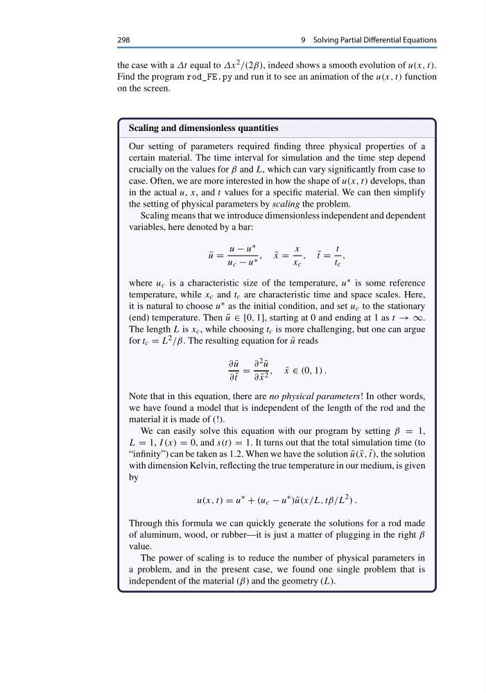
Scaling means that we introduce dimensionless independent and dependent
variables, here denoted by a bar:
¯
u =
u − u ∗
u c − u ∗ , ¯
x =
x
x c
, ¯
t =
t
t c
,
where u c is a characteristic size of the temperature, u ∗ is some reference
temperature, while x c and t c are characteristic time and space scales. Here,
it is natural to choose u ∗ as the initial condition, and set u c to the stationary
(end) temperature. Then ¯
u ∈ [0, 1], starting at 0 and ending at 1 as t → ∞.
The length L is x c , while choosing t c is more challenging, but one can argue
for t c = L 2 /β. The resulting equation for ¯
u reads
∂ ¯
u
∂ ¯
t
=
∂ 2 ¯
u
∂ ¯
x 2 , ¯
x ∈ (0, 1) .
Note that in this equation, there are no physical parameters! In other words,
we have found a model that is independent of the length of the rod and the
material it is made of (!).
We can easily solve this equation with our program by setting β = 1,
L = 1, I (x) = 0, and s(t) = 1. It turns out that the total simulation time (to
“infinity”) can be taken as 1.2. When we have the solution ¯
u( ¯
x, ¯
t), the solution
with dimension Kelvin, reflecting the true temperature in our medium, is given
by
u(x, t) = u
∗
+ (u c − u
∗ ) ¯
u(x/L, tβ/L
2 ) .
Through this formula we can quickly generate the solutions for a rod made
of aluminum, wood, or rubber—it is just a matter of plugging in the right β
value.
The power of scaling is to reduce the number of physical parameters in
a problem, and in the present case, we found one single problem that is
independent of the material (β) and the geometry (L).
9 Solving Partial Differential Equations
the case with a Δt equal to Δx 2 /(2β), indeed shows a smooth evolution of u(x, t).
Find the program rod_FE.py and run it to see an animation of the u(x, t) function
on the screen.
Scaling and dimensionless quantities
Our setting of parameters required finding three physical properties of a
certain material. The time interval for simulation and the time step depend
crucially on the values for β and L, which can vary significantly from case to
case. Often, we are more interested in how the shape of u(x, t) develops, than
in the actual u, x, and t values for a specific material. We can then simplify
the setting of physical parameters by scaling the problem.
Scaling means that we introduce dimensionless independent and dependent
variables, here denoted by a bar:
¯
u =
u − u ∗
u c − u ∗ , ¯
x =
x
x c
, ¯
t =
t
t c
,
where u c is a characteristic size of the temperature, u ∗ is some reference
temperature, while x c and t c are characteristic time and space scales. Here,
it is natural to choose u ∗ as the initial condition, and set u c to the stationary
(end) temperature. Then ¯
u ∈ [0, 1], starting at 0 and ending at 1 as t → ∞.
The length L is x c , while choosing t c is more challenging, but one can argue
for t c = L 2 /β. The resulting equation for ¯
u reads
∂ ¯
u
∂ ¯
t
=
∂ 2 ¯
u
∂ ¯
x 2 , ¯
x ∈ (0, 1) .
Note that in this equation, there are no physical parameters! In other words,
we have found a model that is independent of the length of the rod and the
material it is made of (!).
We can easily solve this equation with our program by setting β = 1,
L = 1, I (x) = 0, and s(t) = 1. It turns out that the total simulation time (to
“infinity”) can be taken as 1.2. When we have the solution ¯
u( ¯
x, ¯
t), the solution
with dimension Kelvin, reflecting the true temperature in our medium, is given
by
u(x, t) = u
∗
+ (u c − u
∗ ) ¯
u(x/L, tβ/L
2 ) .
Through this formula we can quickly generate the solutions for a rod made
of aluminum, wood, or rubber—it is just a matter of plugging in the right β
value.
The power of scaling is to reduce the number of physical parameters in
a problem, and in the present case, we found one single problem that is
independent of the material (β) and the geometry (L).