

9.2 Finite Difference Methods
297
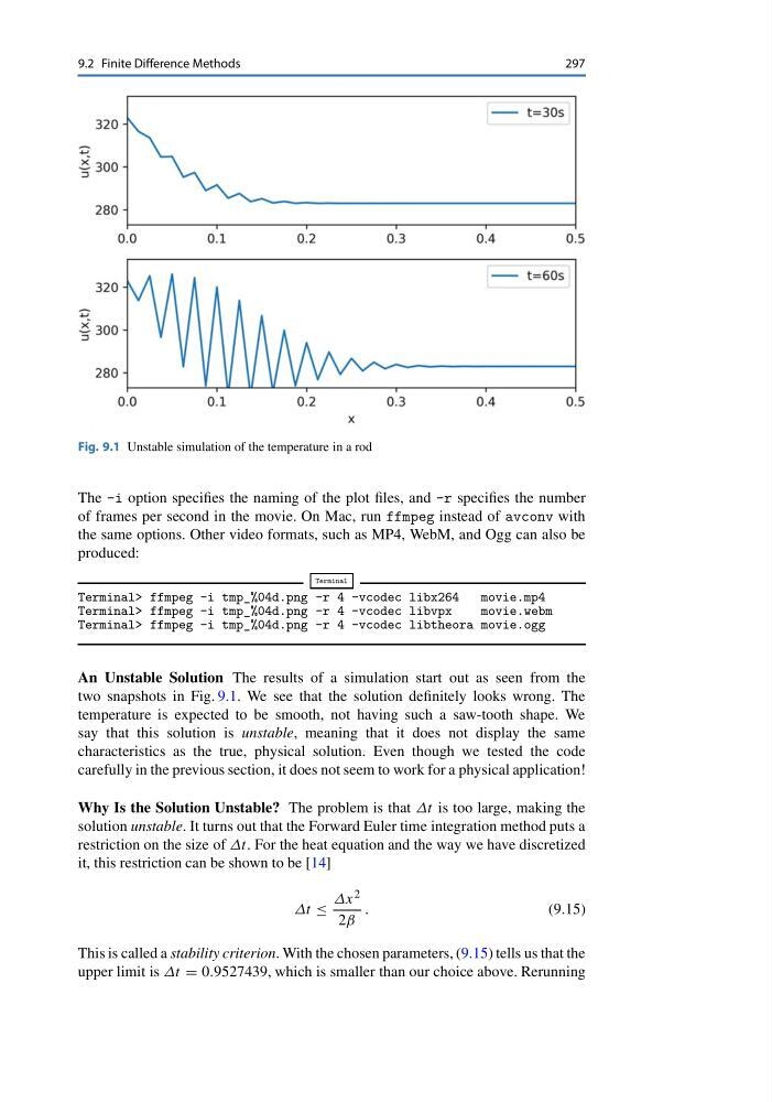
Fig. 9.1 Unstable simulation of the temperature in a rod
The -i option specifies the naming of the plot files, and -r specifies the number
of frames per second in the movie. On Mac, run ffmpeg instead of avconv with
the same options. Other video formats, such as MP4, WebM, and Ogg can also be
produced:
Terminal
Terminal> ffmpeg -i tmp_%04d.png -r 4 -vcodec libx264
movie.mp4
Terminal> ffmpeg -i tmp_%04d.png -r 4 -vcodec libvpx
movie.webm
Terminal> ffmpeg -i tmp_%04d.png -r 4 -vcodec libtheora movie.ogg
An Unstable Solution The results of a simulation start out as seen from the
two snapshots in Fig. 9.1. We see that the solution definitely looks wrong. The
temperature is expected to be smooth, not having such a saw-tooth shape. We
say that this solution is unstable, meaning that it does not display the same
characteristics as the true, physical solution. Even though we tested the code
carefully in the previous section, it does not seem to work for a physical application!
Why Is the Solution Unstable? The problem is that Δt is too large, making the
solution unstable. It turns out that the Forward Euler time integration method puts a
restriction on the size of Δt. For the heat equation and the way we have discretized
it, this restriction can be shown to be [14]
Δt ≤
Δx 2
2β
.
(9.15)
This is called a stability criterion. With the chosen parameters, (9.15) tells us that the
upper limit is Δt = 0.9527439, which is smaller than our choice above. Rerunning
297
Fig. 9.1 Unstable simulation of the temperature in a rod
The -i option specifies the naming of the plot files, and -r specifies the number
of frames per second in the movie. On Mac, run ffmpeg instead of avconv with
the same options. Other video formats, such as MP4, WebM, and Ogg can also be
produced:
Terminal
Terminal> ffmpeg -i tmp_%04d.png -r 4 -vcodec libx264
movie.mp4
Terminal> ffmpeg -i tmp_%04d.png -r 4 -vcodec libvpx
movie.webm
Terminal> ffmpeg -i tmp_%04d.png -r 4 -vcodec libtheora movie.ogg
An Unstable Solution The results of a simulation start out as seen from the
two snapshots in Fig. 9.1. We see that the solution definitely looks wrong. The
temperature is expected to be smooth, not having such a saw-tooth shape. We
say that this solution is unstable, meaning that it does not display the same
characteristics as the true, physical solution. Even though we tested the code
carefully in the previous section, it does not seem to work for a physical application!
Why Is the Solution Unstable? The problem is that Δt is too large, making the
solution unstable. It turns out that the Forward Euler time integration method puts a
restriction on the size of Δt. For the heat equation and the way we have discretized
it, this restriction can be shown to be [14]
Δt ≤
Δx 2
2β
.
(9.15)
This is called a stability criterion. With the chosen parameters, (9.15) tells us that the
upper limit is Δt = 0.9527439, which is smaller than our choice above. Rerunning