

294
9 Solving Partial Differential Equations
for i in range(1, N):
rhs[i] = (beta/dx**2)*(u[i+1] - 2*u[i] + u[i-1]) + \
g(x[i], t)
rhs[N] = (beta/dx**2)*(2*u[N-1] + 2*dx*dudx(t) -
2*u[N]) + g(x[N], t)
return rhs
def u_exact(x, t):
return (3*t + 2)*(x - L)
def dudx(t):
return (3*t + 2)
def s(t):
return u_exact(0, t)
def dsdt(t):
return 3*(-L)
def g(x, t):
return 3*(x-L)
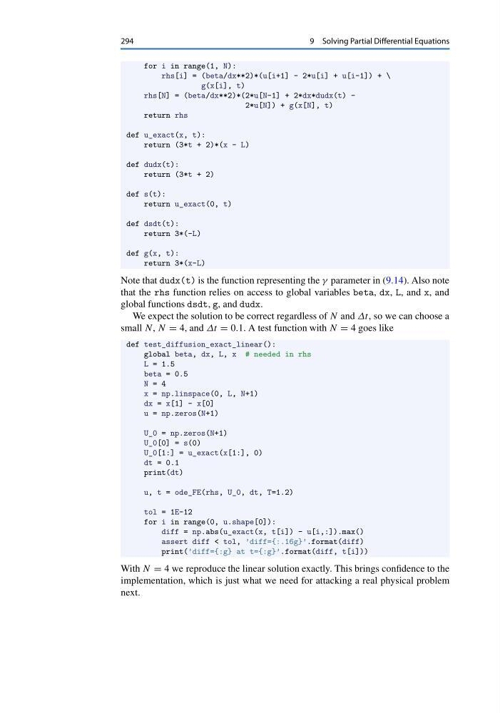
Note that dudx(t) is the function representing the γ parameter in (9.14). Also note
that the rhs function relies on access to global variables beta, dx, L, and x, and
global functions dsdt, g, and dudx.
We expect the solution to be correct regardless of N and Δt, so we can choose a
small N, N = 4, and Δt = 0.1. A test function with N = 4 goes like
def test_diffusion_exact_linear():
global beta, dx, L, x # needed in rhs
L = 1.5
beta = 0.5
N = 4
x = np.linspace(0, L, N+1)
dx = x[1] - x[0]
u = np.zeros(N+1)
U_0 = np.zeros(N+1)
U_0[0] = s(0)
U_0[1:] = u_exact(x[1:], 0)
dt = 0.1
print(dt)
u, t = ode_FE(rhs, U_0, dt, T=1.2)
tol = 1E-12
for i in range(0, u.shape[0]):
diff = np.abs(u_exact(x, t[i]) - u[i,:]).max()
assert diff < tol, ’diff={:.16g}’.format(diff)
print(’diff={:g} at t={:g}’.format(diff, t[i]))
With N = 4 we reproduce the linear solution exactly. This brings confidence to the
implementation, which is just what we need for attacking a real physical problem
next.
9 Solving Partial Differential Equations
for i in range(1, N):
rhs[i] = (beta/dx**2)*(u[i+1] - 2*u[i] + u[i-1]) + \
g(x[i], t)
rhs[N] = (beta/dx**2)*(2*u[N-1] + 2*dx*dudx(t) -
2*u[N]) + g(x[N], t)
return rhs
def u_exact(x, t):
return (3*t + 2)*(x - L)
def dudx(t):
return (3*t + 2)
def s(t):
return u_exact(0, t)
def dsdt(t):
return 3*(-L)
def g(x, t):
return 3*(x-L)
Note that dudx(t) is the function representing the γ parameter in (9.14). Also note
that the rhs function relies on access to global variables beta, dx, L, and x, and
global functions dsdt, g, and dudx.
We expect the solution to be correct regardless of N and Δt, so we can choose a
small N, N = 4, and Δt = 0.1. A test function with N = 4 goes like
def test_diffusion_exact_linear():
global beta, dx, L, x # needed in rhs
L = 1.5
beta = 0.5
N = 4
x = np.linspace(0, L, N+1)
dx = x[1] - x[0]
u = np.zeros(N+1)
U_0 = np.zeros(N+1)
U_0[0] = s(0)
U_0[1:] = u_exact(x[1:], 0)
dt = 0.1
print(dt)
u, t = ode_FE(rhs, U_0, dt, T=1.2)
tol = 1E-12
for i in range(0, u.shape[0]):
diff = np.abs(u_exact(x, t[i]) - u[i,:]).max()
assert diff < tol, ’diff={:.16g}’.format(diff)
print(’diff={:g} at t={:g}’.format(diff, t[i]))
With N = 4 we reproduce the linear solution exactly. This brings confidence to the
implementation, which is just what we need for attacking a real physical problem
next.