

9.2 Finite Difference Methods
293
9.2.2 Construction of a Test Problem with Known Discrete
Solution
At this point, it is tempting to implement a real physical case and run it. However,
PDEs constitute a non-trivial topic where mathematical and programming mistakes
come easy. A better start is therefore to address a carefully designed test example
where we can check that the method works. The most attractive examples for testing
implementations are those without approximation errors, because we know exactly
what numbers the program should produce. It turns out that solutions u(x, t) that are
linear in time and in space can be exactly reproduced by most numerical methods
for PDEs. A candidate solution might be
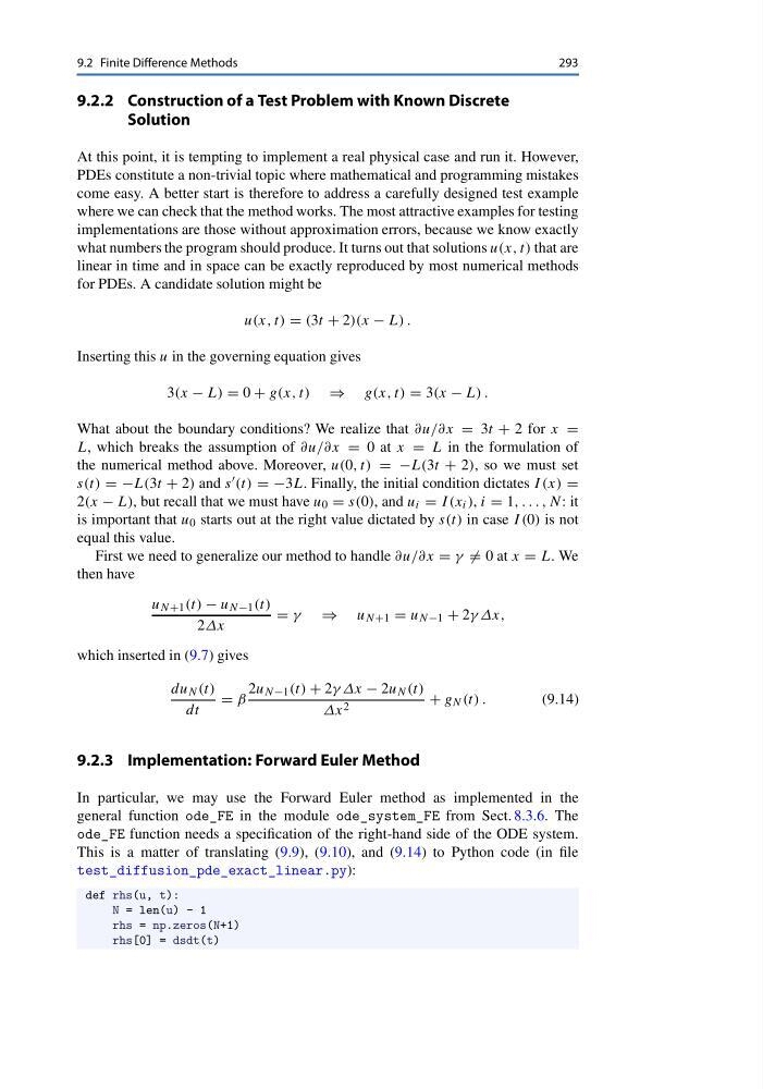
u(x, t) = (3t + 2)(x − L) .
Inserting this u in the governing equation gives
3(x − L) = 0 + g(x, t) ⇒ g(x, t) = 3(x − L) .
What about the boundary conditions? We realize that ∂u/∂x = 3t + 2 for x =
L, which breaks the assumption of ∂u/∂x = 0 at x = L in the formulation of
the numerical method above. Moreover, u(0, t) = −L(3t + 2), so we must set
s(t) = −L(3t + 2) and s (t) = −3L. Finally, the initial condition dictates I (x) =
2(x − L), but recall that we must have u 0 = s(0), and u i = I (x i ), i = 1, . . . , N: it
is important that u 0 starts out at the right value dictated by s(t) in case I (0) is not
equal this value.
First we need to generalize our method to handle ∂u/∂x = γ = 0 at x = L. We
then have
u N+1 (t) − u N−1 (t)
2Δx
= γ ⇒ u N+1 = u N−1 + 2γ Δx,
which inserted in (9.7) gives
du N (t)
dt
= β
2u N−1 (t) + 2γ Δx − 2u N (t)
Δx 2
+ g N (t) .
(9.14)
9.2.3 Implementation: Forward Euler Method
In particular, we may use the Forward Euler method as implemented in the
general function ode_FE in the module ode_system_FE from Sect. 8.3.6. The
ode_FE function needs a specification of the right-hand side of the ODE system.
This is a matter of translating (9.9), (9.10), and (9.14) to Python code (in file
test_diffusion_pde_exact_linear.py):
def rhs(u, t):
N = len(u) - 1
rhs = np.zeros(N+1)
rhs[0] = dsdt(t)
293
9.2.2 Construction of a Test Problem with Known Discrete
Solution
At this point, it is tempting to implement a real physical case and run it. However,
PDEs constitute a non-trivial topic where mathematical and programming mistakes
come easy. A better start is therefore to address a carefully designed test example
where we can check that the method works. The most attractive examples for testing
implementations are those without approximation errors, because we know exactly
what numbers the program should produce. It turns out that solutions u(x, t) that are
linear in time and in space can be exactly reproduced by most numerical methods
for PDEs. A candidate solution might be
u(x, t) = (3t + 2)(x − L) .
Inserting this u in the governing equation gives
3(x − L) = 0 + g(x, t) ⇒ g(x, t) = 3(x − L) .
What about the boundary conditions? We realize that ∂u/∂x = 3t + 2 for x =
L, which breaks the assumption of ∂u/∂x = 0 at x = L in the formulation of
the numerical method above. Moreover, u(0, t) = −L(3t + 2), so we must set
s(t) = −L(3t + 2) and s (t) = −3L. Finally, the initial condition dictates I (x) =
2(x − L), but recall that we must have u 0 = s(0), and u i = I (x i ), i = 1, . . . , N: it
is important that u 0 starts out at the right value dictated by s(t) in case I (0) is not
equal this value.
First we need to generalize our method to handle ∂u/∂x = γ = 0 at x = L. We
then have
u N+1 (t) − u N−1 (t)
2Δx
= γ ⇒ u N+1 = u N−1 + 2γ Δx,
which inserted in (9.7) gives
du N (t)
dt
= β
2u N−1 (t) + 2γ Δx − 2u N (t)
Δx 2
+ g N (t) .
(9.14)
9.2.3 Implementation: Forward Euler Method
In particular, we may use the Forward Euler method as implemented in the
general function ode_FE in the module ode_system_FE from Sect. 8.3.6. The
ode_FE function needs a specification of the right-hand side of the ODE system.
This is a matter of translating (9.9), (9.10), and (9.14) to Python code (in file
test_diffusion_pde_exact_linear.py):
def rhs(u, t):
N = len(u) - 1
rhs = np.zeros(N+1)
rhs[0] = dsdt(t)