

272
8 Solving Ordinary Differential Equations
With (8.87), we have a simple way of computing the error E i , letting
E i = e n l 2 .
(8.88)
We are now in position to compute convergence rates, and write corresponding test
functions, also for ODE solvers.
8.5.3 Test Function: Convergence Rates for the FE Solver
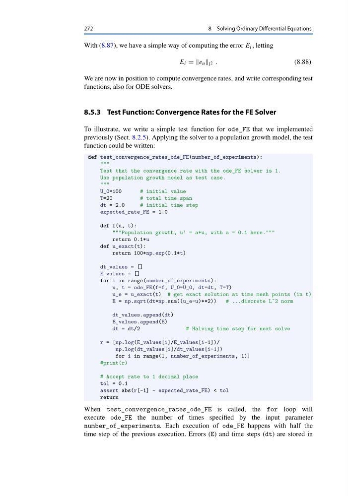
To illustrate, we write a simple test function for ode_FE that we implemented
previously (Sect. 8.2.5). Applying the solver to a population growth model, the test
function could be written:
def test_convergence_rates_ode_FE(number_of_experiments):
"""
Test that the convergence rate with the ode_FE solver is 1.
Use population growth model as test case.
"""
U_0=100
# initial value
T=20
# total time span
dt = 2.0
# initial time step
expected_rate_FE = 1.0
def f(u, t):
"""Population growth, u’ = a*u, with a = 0.1 here."""
return 0.1*u
def u_exact(t):
return 100*np.exp(0.1*t)
dt_values = []
E_values = []
for i in range(number_of_experiments):
u, t = ode_FE(f=f, U_0=U_0, dt=dt, T=T)
u_e = u_exact(t) # get exact solution at time mesh points (in t)
E = np.sqrt(dt*np.sum((u_e-u)**2))
# ...discrete L^2 norm
dt_values.append(dt)
E_values.append(E)
dt = dt/2
# Halving time step for next solve
r = [np.log(E_values[i]/E_values[i-1])/
np.log(dt_values[i]/dt_values[i-1])
for i in range(1, number_of_experiments, 1)]
#print(r)
# Accept rate to 1 decimal place
tol = 0.1
assert abs(r[-1] - expected_rate_FE) < tol
return
When test_convergence_rates_ode_FE is called, the for loop will
execute ode_FE the number of times specified by the input parameter
number_of_experiments. Each execution of ode_FE happens with half the
time step of the previous execution. Errors (E) and time steps (dt) are stored in
8 Solving Ordinary Differential Equations
With (8.87), we have a simple way of computing the error E i , letting
E i = e n l 2 .
(8.88)
We are now in position to compute convergence rates, and write corresponding test
functions, also for ODE solvers.
8.5.3 Test Function: Convergence Rates for the FE Solver
To illustrate, we write a simple test function for ode_FE that we implemented
previously (Sect. 8.2.5). Applying the solver to a population growth model, the test
function could be written:
def test_convergence_rates_ode_FE(number_of_experiments):
"""
Test that the convergence rate with the ode_FE solver is 1.
Use population growth model as test case.
"""
U_0=100
# initial value
T=20
# total time span
dt = 2.0
# initial time step
expected_rate_FE = 1.0
def f(u, t):
"""Population growth, u’ = a*u, with a = 0.1 here."""
return 0.1*u
def u_exact(t):
return 100*np.exp(0.1*t)
dt_values = []
E_values = []
for i in range(number_of_experiments):
u, t = ode_FE(f=f, U_0=U_0, dt=dt, T=T)
u_e = u_exact(t) # get exact solution at time mesh points (in t)
E = np.sqrt(dt*np.sum((u_e-u)**2))
# ...discrete L^2 norm
dt_values.append(dt)
E_values.append(E)
dt = dt/2
# Halving time step for next solve
r = [np.log(E_values[i]/E_values[i-1])/
np.log(dt_values[i]/dt_values[i-1])
for i in range(1, number_of_experiments, 1)]
#print(r)
# Accept rate to 1 decimal place
tol = 0.1
assert abs(r[-1] - expected_rate_FE) < tol
return
When test_convergence_rates_ode_FE is called, the for loop will
execute ode_FE the number of times specified by the input parameter
number_of_experiments. Each execution of ode_FE happens with half the
time step of the previous execution. Errors (E) and time steps (dt) are stored in