

8.5 Rate of Convergence
271
midpoint methods), the error was a single number for each choice of n, i.e., the
number of sub-intervals. With each Δt i now, however, there is basically one error
for each point in the mesh (remember: we compute an approximation to a function
now, not a single number, as we did with integrals)! What we would like to have,
is a single number E i that we could refer to as “the error” of the corresponding
experiment.
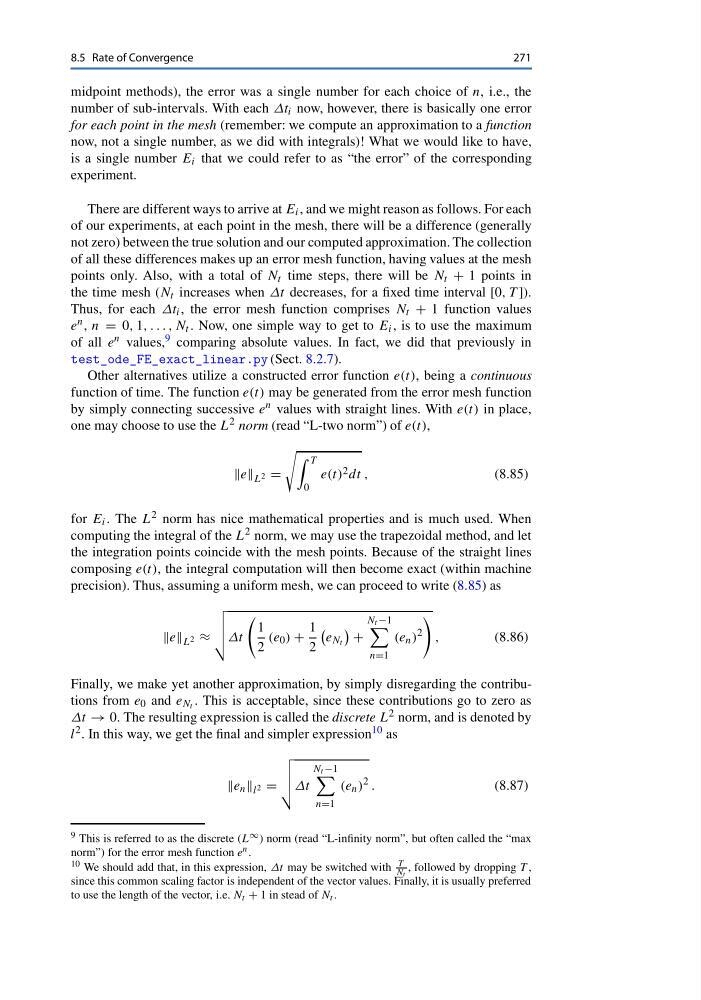
There are different ways to arrive at E i , and we might reason as follows. For each
of our experiments, at each point in the mesh, there will be a difference (generally
not zero) between the true solution and our computed approximation. The collection
of all these differences makes up an error mesh function, having values at the mesh
points only. Also, with a total of N t time steps, there will be N t + 1 points in
the time mesh (N t increases when Δt decreases, for a fixed time interval [0, T ]).
Thus, for each Δt i , the error mesh function comprises N t + 1 function values
e n , n = 0, 1, . . . , N t . Now, one simple way to get to E i , is to use the maximum
of all e n values, 9 comparing absolute values. In fact, we did that previously in
test_ode_FE_exact_linear.py (Sect. 8.2.7).
Other alternatives utilize a constructed error function e(t), being a continuous
function of time. The function e(t) may be generated from the error mesh function
by simply connecting successive e n values with straight lines. With e(t) in place,
one may choose to use the L 2 norm (read “L-two norm”) of e(t),
e L 2 =
T
0
e(t) 2 dt ,
(8.85)
for E i . The L 2 norm has nice mathematical properties and is much used. When
computing the integral of the L 2 norm, we may use the trapezoidal method, and let
the integration points coincide with the mesh points. Because of the straight lines
composing e(t), the integral computation will then become exact (within machine
precision). Thus, assuming a uniform mesh, we can proceed to write (8.85) as
e L 2 ≈
Δt
1
2
(e 0 ) +
1
2
e N t
+
N t −1
n=1
(e n )
2
,
(8.86)
Finally, we make yet another approximation, by simply disregarding the contributions from e 0 and e N t . This is acceptable, since these contributions go to zero as
Δt → 0. The resulting expression is called the discrete L 2 norm, and is denoted by
l 2 . In this way, we get the final and simpler expression 10 as
e n l 2 =
Δt
N t −1
n=1
(e n )
2 .
(8.87)
9 This is referred to as the discrete (L ∞ ) norm (read “L-infinity norm”, but often called the “max
norm”) for the error mesh function e n .
10 We should add that, in this expression, Δt may be switched with
T
Nt , followed by dropping T ,
since this common scaling factor is independent of the vector values. Finally, it is usually preferred
to use the length of the vector, i.e. N t + 1 in stead of N t .
271
midpoint methods), the error was a single number for each choice of n, i.e., the
number of sub-intervals. With each Δt i now, however, there is basically one error
for each point in the mesh (remember: we compute an approximation to a function
now, not a single number, as we did with integrals)! What we would like to have,
is a single number E i that we could refer to as “the error” of the corresponding
experiment.
There are different ways to arrive at E i , and we might reason as follows. For each
of our experiments, at each point in the mesh, there will be a difference (generally
not zero) between the true solution and our computed approximation. The collection
of all these differences makes up an error mesh function, having values at the mesh
points only. Also, with a total of N t time steps, there will be N t + 1 points in
the time mesh (N t increases when Δt decreases, for a fixed time interval [0, T ]).
Thus, for each Δt i , the error mesh function comprises N t + 1 function values
e n , n = 0, 1, . . . , N t . Now, one simple way to get to E i , is to use the maximum
of all e n values, 9 comparing absolute values. In fact, we did that previously in
test_ode_FE_exact_linear.py (Sect. 8.2.7).
Other alternatives utilize a constructed error function e(t), being a continuous
function of time. The function e(t) may be generated from the error mesh function
by simply connecting successive e n values with straight lines. With e(t) in place,
one may choose to use the L 2 norm (read “L-two norm”) of e(t),
e L 2 =
T
0
e(t) 2 dt ,
(8.85)
for E i . The L 2 norm has nice mathematical properties and is much used. When
computing the integral of the L 2 norm, we may use the trapezoidal method, and let
the integration points coincide with the mesh points. Because of the straight lines
composing e(t), the integral computation will then become exact (within machine
precision). Thus, assuming a uniform mesh, we can proceed to write (8.85) as
e L 2 ≈
Δt
1
2
(e 0 ) +
1
2
e N t
+
N t −1
n=1
(e n )
2
,
(8.86)
Finally, we make yet another approximation, by simply disregarding the contributions from e 0 and e N t . This is acceptable, since these contributions go to zero as
Δt → 0. The resulting expression is called the discrete L 2 norm, and is denoted by
l 2 . In this way, we get the final and simpler expression 10 as
e n l 2 =
Δt
N t −1
n=1
(e n )
2 .
(8.87)
9 This is referred to as the discrete (L ∞ ) norm (read “L-infinity norm”, but often called the “max
norm”) for the error mesh function e n .
10 We should add that, in this expression, Δt may be switched with
T
Nt , followed by dropping T ,
since this common scaling factor is independent of the vector values. Finally, it is usually preferred
to use the length of the vector, i.e. N t + 1 in stead of N t .