

230
8 Solving Ordinary Differential Equations
plt.savefig(’tmp.pdf’); plt.savefig(’tmp.png’)
plt.show()
This program was written to investigate the spreading of flu at the mentioned
boarding school, and the reasoning for the specific choices β and γ goes as follows.
At some other school where the disease has already spread, it was observed that
in the beginning of a day there were 40 susceptibles and 8 infected, while the
numbers were 30 and 18, respectively, 24 h later. Using 1 h as time unit, we then
have from (8.11) that β = 10/(40 · 8 · 24). Among 15 infected, it was observed
that 3 recovered during a day, giving γ = 3/(15 · 24). Applying these parameters
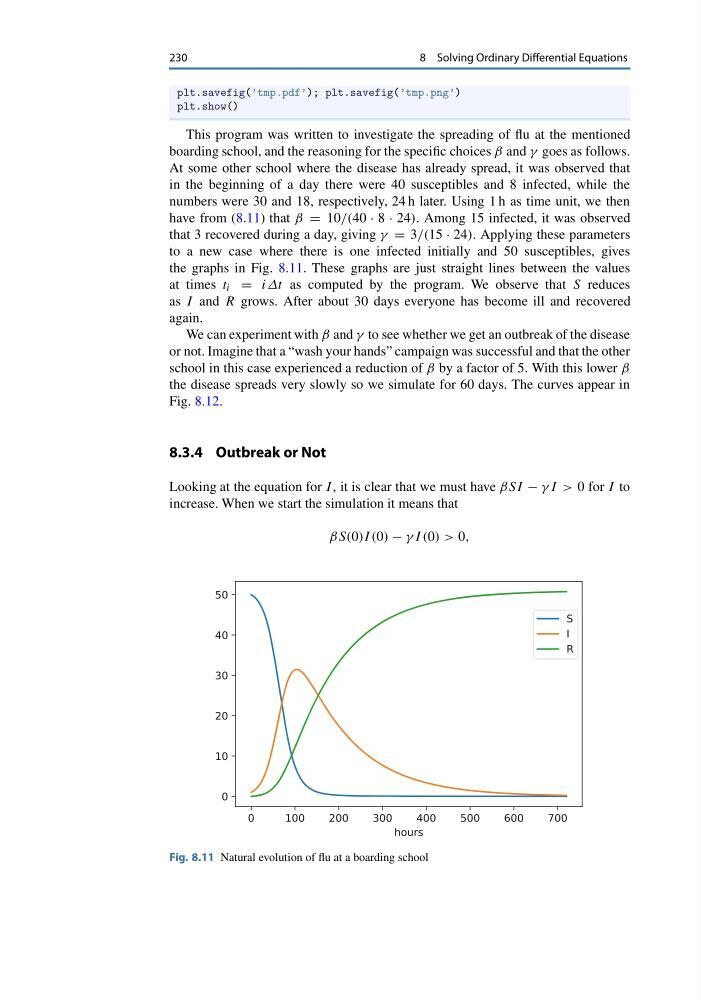
to a new case where there is one infected initially and 50 susceptibles, gives
the graphs in Fig. 8.11. These graphs are just straight lines between the values
at times t i = iΔt as computed by the program. We observe that S reduces
as I and R grows. After about 30 days everyone has become ill and recovered
again.
We can experiment with β and γ to see whether we get an outbreak of the disease
or not. Imagine that a “wash your hands” campaign was successful and that the other
school in this case experienced a reduction of β by a factor of 5. With this lower β
the disease spreads very slowly so we simulate for 60 days. The curves appear in
Fig. 8.12.
8.3.4 Outbreak or Not
Looking at the equation for I , it is clear that we must have βSI − γ I > 0 for I to
increase. When we start the simulation it means that
βS(0)I (0) − γ I (0) > 0,
Fig. 8.11 Natural evolution of flu at a boarding school
8 Solving Ordinary Differential Equations
plt.savefig(’tmp.pdf’); plt.savefig(’tmp.png’)
plt.show()
This program was written to investigate the spreading of flu at the mentioned
boarding school, and the reasoning for the specific choices β and γ goes as follows.
At some other school where the disease has already spread, it was observed that
in the beginning of a day there were 40 susceptibles and 8 infected, while the
numbers were 30 and 18, respectively, 24 h later. Using 1 h as time unit, we then
have from (8.11) that β = 10/(40 · 8 · 24). Among 15 infected, it was observed
that 3 recovered during a day, giving γ = 3/(15 · 24). Applying these parameters
to a new case where there is one infected initially and 50 susceptibles, gives
the graphs in Fig. 8.11. These graphs are just straight lines between the values
at times t i = iΔt as computed by the program. We observe that S reduces
as I and R grows. After about 30 days everyone has become ill and recovered
again.
We can experiment with β and γ to see whether we get an outbreak of the disease
or not. Imagine that a “wash your hands” campaign was successful and that the other
school in this case experienced a reduction of β by a factor of 5. With this lower β
the disease spreads very slowly so we simulate for 60 days. The curves appear in
Fig. 8.12.
8.3.4 Outbreak or Not
Looking at the equation for I , it is clear that we must have βSI − γ I > 0 for I to
increase. When we start the simulation it means that
βS(0)I (0) − γ I (0) > 0,
Fig. 8.11 Natural evolution of flu at a boarding school