

8.3 Spreading of Disease: A System of First Order ODEs
229
for n = 0, 1, . . . , N t . This is an approximation since the differential equations are
originally valid at all times t (usually in some finite interval [0, T ]). Using forward
finite differences for the derivatives results in an additional approximation,
S n+1 − S n
Δt
= −βS
n I
n ,
(8.26)
I n+1 − I n
Δt
= βS
n I
n
− γ I
n ,
(8.27)
R n+1 − R n
Δt
= γ I
n .
(8.28)
As we can see, these equations are identical to the difference equations that
naturally arise in the derivation of the model. However, other numerical methods
than the Forward Euler scheme will result in slightly different difference equations.
8.3.3 Programming the FE Scheme; the Special Case
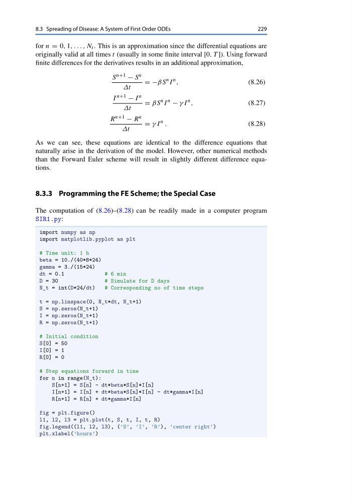
The computation of (8.26)–(8.28) can be readily made in a computer program
SIR1.py:
import numpy as np
import matplotlib.pyplot as plt
# Time unit: 1 h
beta = 10./(40*8*24)
gamma = 3./(15*24)
dt = 0.1
# 6 min
D = 30
# Simulate for D days
N_t = int(D*24/dt)
# Corresponding no of time steps
t = np.linspace(0, N_t*dt, N_t+1)
S = np.zeros(N_t+1)
I = np.zeros(N_t+1)
R = np.zeros(N_t+1)
# Initial condition
S[0] = 50
I[0] = 1
R[0] = 0
# Step equations forward in time
for n in range(N_t):
S[n+1] = S[n] - dt*beta*S[n]*I[n]
I[n+1] = I[n] + dt*beta*S[n]*I[n] - dt*gamma*I[n]
R[n+1] = R[n] + dt*gamma*I[n]
fig = plt.figure()
l1, l2, l3 = plt.plot(t, S, t, I, t, R)
fig.legend((l1, l2, l3), (’S’, ’I’, ’R’), ’center right’)
plt.xlabel(’hours’)
229
for n = 0, 1, . . . , N t . This is an approximation since the differential equations are
originally valid at all times t (usually in some finite interval [0, T ]). Using forward
finite differences for the derivatives results in an additional approximation,
S n+1 − S n
Δt
= −βS
n I
n ,
(8.26)
I n+1 − I n
Δt
= βS
n I
n
− γ I
n ,
(8.27)
R n+1 − R n
Δt
= γ I
n .
(8.28)
As we can see, these equations are identical to the difference equations that
naturally arise in the derivation of the model. However, other numerical methods
than the Forward Euler scheme will result in slightly different difference equations.
8.3.3 Programming the FE Scheme; the Special Case
The computation of (8.26)–(8.28) can be readily made in a computer program
SIR1.py:
import numpy as np
import matplotlib.pyplot as plt
# Time unit: 1 h
beta = 10./(40*8*24)
gamma = 3./(15*24)
dt = 0.1
# 6 min
D = 30
# Simulate for D days
N_t = int(D*24/dt)
# Corresponding no of time steps
t = np.linspace(0, N_t*dt, N_t+1)
S = np.zeros(N_t+1)
I = np.zeros(N_t+1)
R = np.zeros(N_t+1)
# Initial condition
S[0] = 50
I[0] = 1
R[0] = 0
# Step equations forward in time
for n in range(N_t):
S[n+1] = S[n] - dt*beta*S[n]*I[n]
I[n+1] = I[n] + dt*beta*S[n]*I[n] - dt*gamma*I[n]
R[n+1] = R[n] + dt*gamma*I[n]
fig = plt.figure()
l1, l2, l3 = plt.plot(t, S, t, I, t, R)
fig.legend((l1, l2, l3), (’S’, ’I’, ’R’), ’center right’)
plt.xlabel(’hours’)