

218
8 Solving Ordinary Differential Equations
Note the compact assignment statement
numerical_sol = ’bo’ if N_t < 70 else ’b-’
This is a one-line alternative to, e.g.,
if N_t < 70:
numerical_sol = ’bo’
else:
numerical_sol = ’b-’
Let us demonstrate a simulation where we start with 100 animals, a net growth
rate of 10% (0.1) per time unit, which can be 1 month, and t ∈ [0, 20] months. We
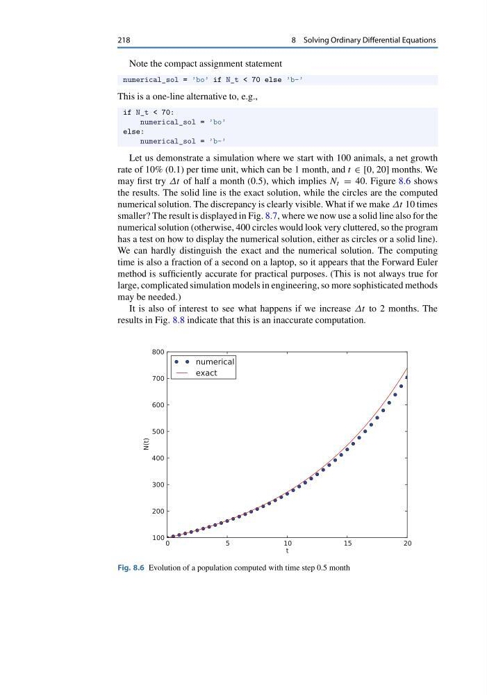
may first try Δt of half a month (0.5), which implies N t = 40. Figure 8.6 shows
the results. The solid line is the exact solution, while the circles are the computed
numerical solution. The discrepancy is clearly visible. What if we make Δt 10 times
smaller? The result is displayed in Fig. 8.7, where we now use a solid line also for the
numerical solution (otherwise, 400 circles would look very cluttered, so the program
has a test on how to display the numerical solution, either as circles or a solid line).
We can hardly distinguish the exact and the numerical solution. The computing
time is also a fraction of a second on a laptop, so it appears that the Forward Euler
method is sufficiently accurate for practical purposes. (This is not always true for
large, complicated simulation models in engineering, so more sophisticated methods
may be needed.)
It is also of interest to see what happens if we increase Δt to 2 months. The
results in Fig. 8.8 indicate that this is an inaccurate computation.
Fig. 8.6 Evolution of a population computed with time step 0.5 month
8 Solving Ordinary Differential Equations
Note the compact assignment statement
numerical_sol = ’bo’ if N_t < 70 else ’b-’
This is a one-line alternative to, e.g.,
if N_t < 70:
numerical_sol = ’bo’
else:
numerical_sol = ’b-’
Let us demonstrate a simulation where we start with 100 animals, a net growth
rate of 10% (0.1) per time unit, which can be 1 month, and t ∈ [0, 20] months. We
may first try Δt of half a month (0.5), which implies N t = 40. Figure 8.6 shows
the results. The solid line is the exact solution, while the circles are the computed
numerical solution. The discrepancy is clearly visible. What if we make Δt 10 times
smaller? The result is displayed in Fig. 8.7, where we now use a solid line also for the
numerical solution (otherwise, 400 circles would look very cluttered, so the program
has a test on how to display the numerical solution, either as circles or a solid line).
We can hardly distinguish the exact and the numerical solution. The computing
time is also a fraction of a second on a laptop, so it appears that the Forward Euler
method is sufficiently accurate for practical purposes. (This is not always true for
large, complicated simulation models in engineering, so more sophisticated methods
may be needed.)
It is also of interest to see what happens if we increase Δt to 2 months. The
results in Fig. 8.8 indicate that this is an inaccurate computation.
Fig. 8.6 Evolution of a population computed with time step 0.5 month