

8.2 Population Growth: A First Order ODE
217
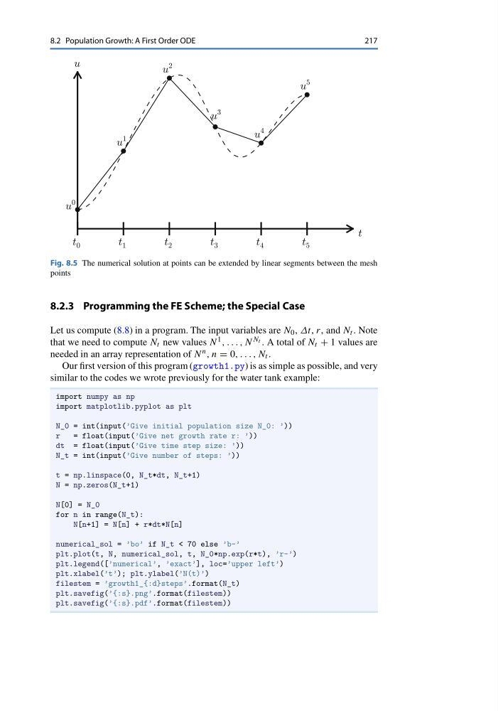
Fig. 8.5 The numerical solution at points can be extended by linear segments between the mesh
points
8.2.3 Programming the FE Scheme; the Special Case
Let us compute (8.8) in a program. The input variables are N 0 , Δt, r, and N t . Note
that we need to compute N t new values N 1 , . . . , N N t . A total of N t + 1 values are
needed in an array representation of N n , n = 0, . . . , N t .
Our first version of this program (growth1.py) is as simple as possible, and very
similar to the codes we wrote previously for the water tank example:
import numpy as np
import matplotlib.pyplot as plt
N_0 = int(input(’Give initial population size N_0: ’))
r
= float(input(’Give net growth rate r: ’))
dt = float(input(’Give time step size: ’))
N_t = int(input(’Give number of steps: ’))
t = np.linspace(0, N_t*dt, N_t+1)
N = np.zeros(N_t+1)
N[0] = N_0
for n in range(N_t):
N[n+1] = N[n] + r*dt*N[n]
numerical_sol = ’bo’ if N_t < 70 else ’b-’
plt.plot(t, N, numerical_sol, t, N_0*np.exp(r*t), ’r-’)
plt.legend([’numerical’, ’exact’], loc=’upper left’)
plt.xlabel(’t’); plt.ylabel(’N(t)’)
filestem = ’growth1_{:d}steps’.format(N_t)
plt.savefig(’{:s}.png’.format(filestem))
plt.savefig(’{:s}.pdf’.format(filestem))
217
Fig. 8.5 The numerical solution at points can be extended by linear segments between the mesh
points
8.2.3 Programming the FE Scheme; the Special Case
Let us compute (8.8) in a program. The input variables are N 0 , Δt, r, and N t . Note
that we need to compute N t new values N 1 , . . . , N N t . A total of N t + 1 values are
needed in an array representation of N n , n = 0, . . . , N t .
Our first version of this program (growth1.py) is as simple as possible, and very
similar to the codes we wrote previously for the water tank example:
import numpy as np
import matplotlib.pyplot as plt
N_0 = int(input(’Give initial population size N_0: ’))
r
= float(input(’Give net growth rate r: ’))
dt = float(input(’Give time step size: ’))
N_t = int(input(’Give number of steps: ’))
t = np.linspace(0, N_t*dt, N_t+1)
N = np.zeros(N_t+1)
N[0] = N_0
for n in range(N_t):
N[n+1] = N[n] + r*dt*N[n]
numerical_sol = ’bo’ if N_t < 70 else ’b-’
plt.plot(t, N, numerical_sol, t, N_0*np.exp(r*t), ’r-’)
plt.legend([’numerical’, ’exact’], loc=’upper left’)
plt.xlabel(’t’); plt.ylabel(’N(t)’)
filestem = ’growth1_{:d}steps’.format(N_t)
plt.savefig(’{:s}.png’.format(filestem))
plt.savefig(’{:s}.pdf’.format(filestem))