

214
8 Solving Ordinary Differential Equations
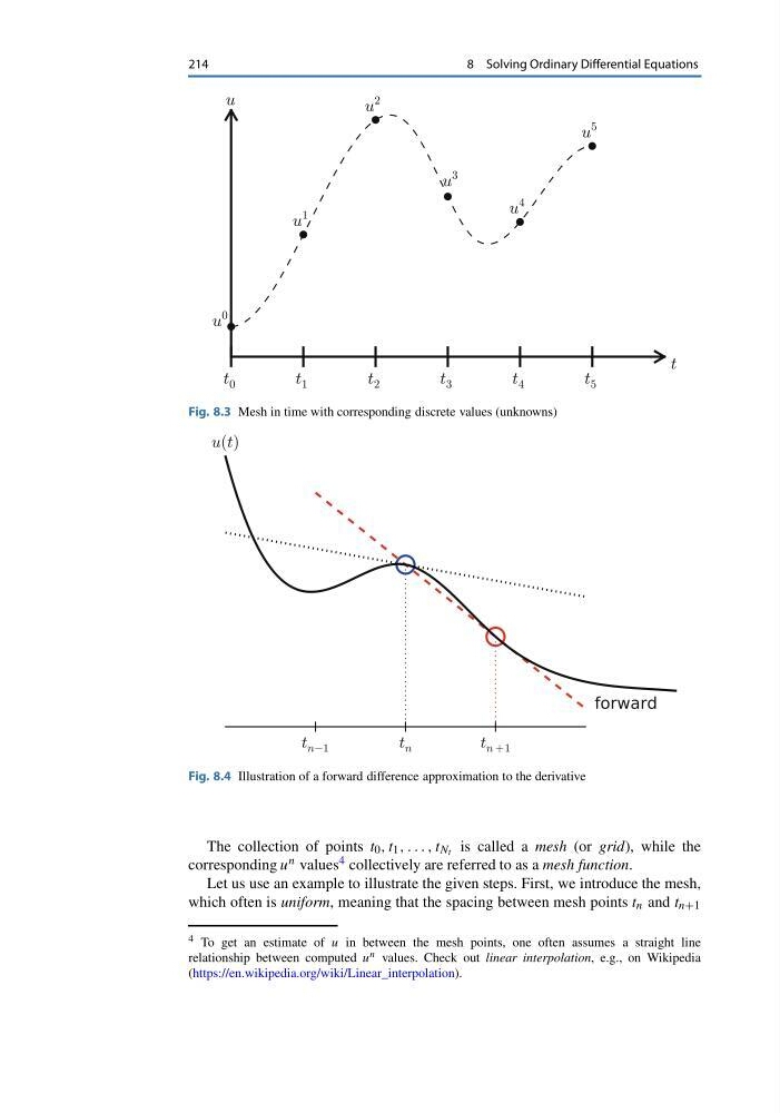
Fig. 8.3 Mesh in time with corresponding discrete values (unknowns)
Fig. 8.4 Illustration of a forward difference approximation to the derivative
The collection of points t 0 , t 1 , . . . , t N t is called a mesh (or grid), while the
corresponding u n values 4 collectively are referred to as a mesh function.
Let us use an example to illustrate the given steps. First, we introduce the mesh,
which often is uniform, meaning that the spacing between mesh points t n and t n+1
4 To get an estimate of u in between the mesh points, one often assumes a straight line
relationship between computed u n values. Check out linear interpolation, e.g., on Wikipedia
(https://en.wikipedia.org/wiki/Linear_interpolation).
8 Solving Ordinary Differential Equations
Fig. 8.3 Mesh in time with corresponding discrete values (unknowns)
Fig. 8.4 Illustration of a forward difference approximation to the derivative
The collection of points t 0 , t 1 , . . . , t N t is called a mesh (or grid), while the
corresponding u n values 4 collectively are referred to as a mesh function.
Let us use an example to illustrate the given steps. First, we introduce the mesh,
which often is uniform, meaning that the spacing between mesh points t n and t n+1
4 To get an estimate of u in between the mesh points, one often assumes a straight line
relationship between computed u n values. Check out linear interpolation, e.g., on Wikipedia
(https://en.wikipedia.org/wiki/Linear_interpolation).