

8.2 Population Growth: A First Order ODE
213
Detour: Exact mathematical solution
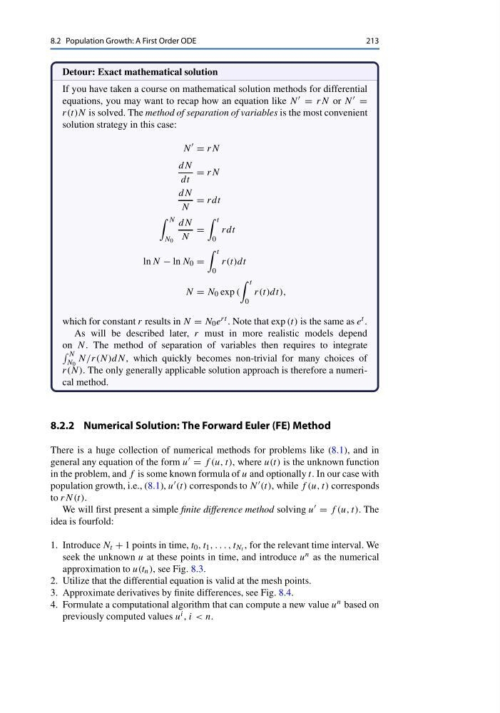
If you have taken a course on mathematical solution methods for differential
equations, you may want to recap how an equation like N = rN or N =
r(t)N is solved. The method of separation of variables is the most convenient
solution strategy in this case:
N
= rN
dN
dt
= rN
dN
N
= rdt
N
N 0
dN
N
=
t
0
rdt
ln N − ln N 0 =
t
0
r(t)dt
N = N 0 exp (
t
0
r(t)dt),
which for constant r results in N = N 0 e rt . Note that exp (t) is the same as e t .
As will be described later, r must in more realistic models depend
on N. The method of separation of variables then requires to integrate
N
N 0
N/r(N)dN, which quickly becomes non-trivial for many choices of
r(N). The only generally applicable solution approach is therefore a numerical method.
8.2.2 Numerical Solution: The Forward Euler (FE) Method
There is a huge collection of numerical methods for problems like (8.1), and in
general any equation of the form u = f (u, t), where u(t) is the unknown function
in the problem, and f is some known formula of u and optionally t. In our case with
population growth, i.e., (8.1), u (t) corresponds to N (t), while f (u, t) corresponds
to rN(t).
We will first present a simple finite difference method solving u = f (u, t). The
idea is fourfold:
1. Introduce N t + 1 points in time, t 0 , t 1 , . . . , t N t , for the relevant time interval. We
seek the unknown u at these points in time, and introduce u n as the numerical
approximation to u(t n ), see Fig. 8.3.
2. Utilize that the differential equation is valid at the mesh points.
3. Approximate derivatives by finite differences, see Fig. 8.4.
4. Formulate a computational algorithm that can compute a new value u n based on
previously computed values u i , i < n.
213
Detour: Exact mathematical solution
If you have taken a course on mathematical solution methods for differential
equations, you may want to recap how an equation like N = rN or N =
r(t)N is solved. The method of separation of variables is the most convenient
solution strategy in this case:
N
= rN
dN
dt
= rN
dN
N
= rdt
N
N 0
dN
N
=
t
0
rdt
ln N − ln N 0 =
t
0
r(t)dt
N = N 0 exp (
t
0
r(t)dt),
which for constant r results in N = N 0 e rt . Note that exp (t) is the same as e t .
As will be described later, r must in more realistic models depend
on N. The method of separation of variables then requires to integrate
N
N 0
N/r(N)dN, which quickly becomes non-trivial for many choices of
r(N). The only generally applicable solution approach is therefore a numerical method.
8.2.2 Numerical Solution: The Forward Euler (FE) Method
There is a huge collection of numerical methods for problems like (8.1), and in
general any equation of the form u = f (u, t), where u(t) is the unknown function
in the problem, and f is some known formula of u and optionally t. In our case with
population growth, i.e., (8.1), u (t) corresponds to N (t), while f (u, t) corresponds
to rN(t).
We will first present a simple finite difference method solving u = f (u, t). The
idea is fourfold:
1. Introduce N t + 1 points in time, t 0 , t 1 , . . . , t N t , for the relevant time interval. We
seek the unknown u at these points in time, and introduce u n as the numerical
approximation to u(t n ), see Fig. 8.3.
2. Utilize that the differential equation is valid at the mesh points.
3. Approximate derivatives by finite differences, see Fig. 8.4.
4. Formulate a computational algorithm that can compute a new value u n based on
previously computed values u i , i < n.