

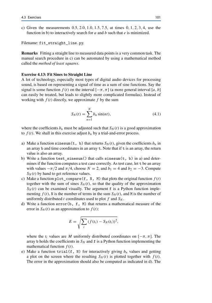
4.3 Exercises
101
c) Given the measurements 0.5, 2.0, 1.0, 1.5, 7.5, at times 0, 1, 2, 3, 4, use the
function in b) to interactively search for a and b such that e is minimized.
Filename: fit_straight_line.py.
Remarks Fitting a straight line to measured data points is a very common task. The
manual search procedure in c) can be automated by using a mathematical method
called the method of least squares.
Exercise 4.13: Fit Sines to Straight Line
A lot of technology, especially most types of digital audio devices for processing
sound, is based on representing a signal of time as a sum of sine functions. Say the
signal is some function f (t) on the interval [−π, π] (a more general interval [a, b]
can easily be treated, but leads to slightly more complicated formulas). Instead of
working with f (t) directly, we approximate f by the sum
S N (t) =
N
n=1
b n sin(nt),
(4.1)
where the coefficients b n must be adjusted such that S N (t) is a good approximation
to f (t). We shall in this exercise adjust b n by a trial-and-error process.
a) Make a function sinesum(t, b) that returns S N (t), given the coefficients b n in
an array b and time coordinates in an array t. Note that if t is an array, the return
value is also an array.
b) Write a function test_sinesum() that calls sinesum(t, b) in a) and determines if the function computes a test case correctly. As test case, let t be an array
with values −π/2 and π/4, choose N = 2, and b 1 = 4 and b 2 = −3. Compute
S N (t) by hand to get reference values.
c) Make a function plot_compare(f, N, M) that plots the original function f (t)
together with the sum of sines S N (t), so that the quality of the approximation
S N (t) can be examined visually. The argument f is a Python function implementing f (t), N is the number of terms in the sum S N (t), and M is the number of
uniformly distributed t coordinates used to plot f and S N .
d) Write a function error(b, f, M) that returns a mathematical measure of the
error in S N (t) as an approximation to f (t):
E =
i
(f (t i ) − S N (t i ))
2 ,
where the t i values are M uniformly distributed coordinates on [−π, π]. The
array b holds the coefficients in S N and f is a Python function implementing the
mathematical function f (t).
e) Make a function trial(f, N) for interactively giving b n values and getting
a plot on the screen where the resulting S N (t) is plotted together with f (t).
The error in the approximation should also be computed as indicated in d). The
101
c) Given the measurements 0.5, 2.0, 1.0, 1.5, 7.5, at times 0, 1, 2, 3, 4, use the
function in b) to interactively search for a and b such that e is minimized.
Filename: fit_straight_line.py.
Remarks Fitting a straight line to measured data points is a very common task. The
manual search procedure in c) can be automated by using a mathematical method
called the method of least squares.
Exercise 4.13: Fit Sines to Straight Line
A lot of technology, especially most types of digital audio devices for processing
sound, is based on representing a signal of time as a sum of sine functions. Say the
signal is some function f (t) on the interval [−π, π] (a more general interval [a, b]
can easily be treated, but leads to slightly more complicated formulas). Instead of
working with f (t) directly, we approximate f by the sum
S N (t) =
N
n=1
b n sin(nt),
(4.1)
where the coefficients b n must be adjusted such that S N (t) is a good approximation
to f (t). We shall in this exercise adjust b n by a trial-and-error process.
a) Make a function sinesum(t, b) that returns S N (t), given the coefficients b n in
an array b and time coordinates in an array t. Note that if t is an array, the return
value is also an array.
b) Write a function test_sinesum() that calls sinesum(t, b) in a) and determines if the function computes a test case correctly. As test case, let t be an array
with values −π/2 and π/4, choose N = 2, and b 1 = 4 and b 2 = −3. Compute
S N (t) by hand to get reference values.
c) Make a function plot_compare(f, N, M) that plots the original function f (t)
together with the sum of sines S N (t), so that the quality of the approximation
S N (t) can be examined visually. The argument f is a Python function implementing f (t), N is the number of terms in the sum S N (t), and M is the number of
uniformly distributed t coordinates used to plot f and S N .
d) Write a function error(b, f, M) that returns a mathematical measure of the
error in S N (t) as an approximation to f (t):
E =
i
(f (t i ) − S N (t i ))
2 ,
where the t i values are M uniformly distributed coordinates on [−π, π]. The
array b holds the coefficients in S N and f is a Python function implementing the
mathematical function f (t).
e) Make a function trial(f, N) for interactively giving b n values and getting
a plot on the screen where the resulting S N (t) is plotted together with f (t).
The error in the approximation should also be computed as indicated in d). The