

476
C. E. Budde et al.
holds nicely for the biggest case studies: HECS 5
† (a 42-nodes rft whose iosa
has 126-not-clock variables ≈ 2.89×10
38 states, with 57 clocks of exponential,
uniform, and log-normal pdfs) and RWC 4 (42 nodes, 181 variables ≈ 6.93×10
73
states, 62 clocks of exponential, Erlang, Rayleigh, uniform, and normal pdfs).
Using smc, restart, and fe, we also estimated UNREL 1000 for RWC 2,3,4 ,
DSPARE 3,4,5 , FTPP 4,5,6 , HVC 4,5,6,7 , and HECS 2,3,4,5 . For HVC (only) we ran
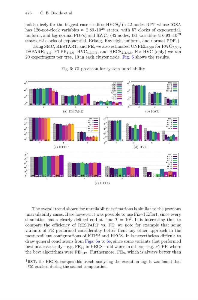
20 experiments per tree, 10 in each cluster node. Fig. 6 shows the results.
Fig. 6: ci precision for system unreliability
(e) HECS
The overall trend shown for unreliability estimations is similar to the previous
unavailability cases. Here however it was possible to use Fixed Effort, since every
simulation has a clearly defined end at time T = 10
3 . It is interesting thus to
compare the efficiency of restart vs. fe: we note for example that some
variants of fe performed considerably better than any other approach in the
most resilient configurations of FTPP and HECS. It is nevertheless difficult to
draw general conclusions from Figs. 6a to 6e, since some variants that performed
best in a case study—e.g. fe 16 in HECS—did worse in others—e.g. FTPP, where
the best algorithms were fe 8,12 . Furthermore, fe 8 , which is always better than
† rst8 for HECS5 escapes this trend: analysing the execution logs it was found that
FIG crashed during the second computation.
(a) DSPARE
(b) RWC
(c) FTPP
1 e - 6
1 e - 5
1 e - 4
1 e - 3
1 e - 2
1 e - 1
4
5
6
7
SMC
10
10
6
6
RST 2
16
15
15
12
RST 5
15
19
16
17
RST 8
19
17
16
13
RST 11
18
18
18
15
FE 8
0
6
1 4
1 0
(d) HVC
1 e - 7
1 e - 6
1 e - 5
1 e - 4
1 e - 3
1 e - 2
2
3
4
5
SMC
10
10
8
1
RST 2
10
10
7
3
RST 5
10
10
10
0
RST 8
10
10
8
1
RST 11
10
10
6
1
FE 8
10
10
10
9
FE 16
10
10
10
10
FE 32
10
10
1
1
C. E. Budde et al.
holds nicely for the biggest case studies: HECS 5
† (a 42-nodes rft whose iosa
has 126-not-clock variables ≈ 2.89×10
38 states, with 57 clocks of exponential,
uniform, and log-normal pdfs) and RWC 4 (42 nodes, 181 variables ≈ 6.93×10
73
states, 62 clocks of exponential, Erlang, Rayleigh, uniform, and normal pdfs).
Using smc, restart, and fe, we also estimated UNREL 1000 for RWC 2,3,4 ,
DSPARE 3,4,5 , FTPP 4,5,6 , HVC 4,5,6,7 , and HECS 2,3,4,5 . For HVC (only) we ran
20 experiments per tree, 10 in each cluster node. Fig. 6 shows the results.
Fig. 6: ci precision for system unreliability
(e) HECS
The overall trend shown for unreliability estimations is similar to the previous
unavailability cases. Here however it was possible to use Fixed Effort, since every
simulation has a clearly defined end at time T = 10
3 . It is interesting thus to
compare the efficiency of restart vs. fe: we note for example that some
variants of fe performed considerably better than any other approach in the
most resilient configurations of FTPP and HECS. It is nevertheless difficult to
draw general conclusions from Figs. 6a to 6e, since some variants that performed
best in a case study—e.g. fe 16 in HECS—did worse in others—e.g. FTPP, where
the best algorithms were fe 8,12 . Furthermore, fe 8 , which is always better than
† rst8 for HECS5 escapes this trend: analysing the execution logs it was found that
FIG crashed during the second computation.
(a) DSPARE
(b) RWC
(c) FTPP
1 e - 6
1 e - 5
1 e - 4
1 e - 3
1 e - 2
1 e - 1
4
5
6
7
SMC
10
10
6
6
RST 2
16
15
15
12
RST 5
15
19
16
17
RST 8
19
17
16
13
RST 11
18
18
18
15
FE 8
0
6
1 4
1 0
(d) HVC
1 e - 7
1 e - 6
1 e - 5
1 e - 4
1 e - 3
1 e - 2
2
3
4
5
SMC
10
10
8
1
RST 2
10
10
7
3
RST 5
10
10
10
0
RST 8
10
10
8
1
RST 11
10
10
6
1
FE 8
10
10
10
9
FE 16
10
10
10
10
FE 32
10
10
1
1