

RES for non-Markovian repairable fault trees
475
5.2 Experimental results and discussion
Using smc and restart we computed UNAVA for VOT 2,3,4 , HECS 1,...,5 ,
RC 3,...,6 , and RWC 1,...,4 . fe was not used since it requires regeneration theory
for steady-state analysis [19], which is not always feasible with non-Markovian
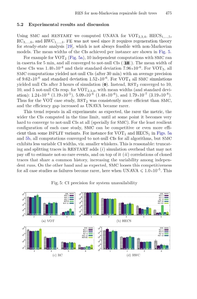
models. The mean widths of the cis achieved per instance are shown in Fig. 5.
For example for VOT 2 (Fig. 5a), 10 independent computations with smc ran
in caserta for 5 min, and all converged to not-null cis ( 10 ). The mean width of
these cis was 1.40×10
-4 and their standard deviation 7.96×10
-6 . For VOT 3 , all
smc computations yielded not-null cis (after 30 min) with an average precision
of 9.62×10
-6 and standard deviation 1.52×10
-6 . For VOT 4 all smc simulations
yielded null cis after 3 hours of simulation (0). Instead, rst 2 converged to 10,
10, and 5 not-null cis resp. for VOT 2,3,4 , with mean widths (and standard deviation): 1.24×10
-4 (1.19×10
-5 ), 5.09×10
-6 (1.48×10
-6 ), and 1.79×10
-7 (3.19×10
-8 ).
Thus for the VOT case study, rst 2 was consistently more efficient than smc,
and the efficiency gap increased as UNAVA became rarer.
This trend repeats in all experiments: as expected, the rarer the metric, the
wider the cis computed in the time limit, until at some point it becomes very
hard to converge to not-null cis at all (specially for smc). For the least resilient
configuration of each case study, smc can be competitive or even more efficient than some isplit variants. For instance for VOT 1 and HECS 1 in Figs. 5a
and 5b, all computations converged to not-null cis for all algorithms, but smc
exhibits less variable ci widths, viz. smaller whiskers. This is reasonable: truncating and splitting traces in restart adds (i ) simulation overhead that may not
pay off to estimate not-so-rare events, and on top of it (ii ) correlations of cloned
traces that share a common history, increasing the variability among independent runs. On the other hand and as expected, smc looses this competitiveness
for all case studies as failures become rarer, here when UNAVA 1.0×10
-5 . This
Fig. 5: ci precision for system unavailability
(a) VOT
(b) HECS
(c) RC
(d) RWC
475
5.2 Experimental results and discussion
Using smc and restart we computed UNAVA for VOT 2,3,4 , HECS 1,...,5 ,
RC 3,...,6 , and RWC 1,...,4 . fe was not used since it requires regeneration theory
for steady-state analysis [19], which is not always feasible with non-Markovian
models. The mean widths of the cis achieved per instance are shown in Fig. 5.
For example for VOT 2 (Fig. 5a), 10 independent computations with smc ran
in caserta for 5 min, and all converged to not-null cis ( 10 ). The mean width of
these cis was 1.40×10
-4 and their standard deviation 7.96×10
-6 . For VOT 3 , all
smc computations yielded not-null cis (after 30 min) with an average precision
of 9.62×10
-6 and standard deviation 1.52×10
-6 . For VOT 4 all smc simulations
yielded null cis after 3 hours of simulation (0). Instead, rst 2 converged to 10,
10, and 5 not-null cis resp. for VOT 2,3,4 , with mean widths (and standard deviation): 1.24×10
-4 (1.19×10
-5 ), 5.09×10
-6 (1.48×10
-6 ), and 1.79×10
-7 (3.19×10
-8 ).
Thus for the VOT case study, rst 2 was consistently more efficient than smc,
and the efficiency gap increased as UNAVA became rarer.
This trend repeats in all experiments: as expected, the rarer the metric, the
wider the cis computed in the time limit, until at some point it becomes very
hard to converge to not-null cis at all (specially for smc). For the least resilient
configuration of each case study, smc can be competitive or even more efficient than some isplit variants. For instance for VOT 1 and HECS 1 in Figs. 5a
and 5b, all computations converged to not-null cis for all algorithms, but smc
exhibits less variable ci widths, viz. smaller whiskers. This is reasonable: truncating and splitting traces in restart adds (i ) simulation overhead that may not
pay off to estimate not-so-rare events, and on top of it (ii ) correlations of cloned
traces that share a common history, increasing the variability among independent runs. On the other hand and as expected, smc looses this competitiveness
for all case studies as failures become rarer, here when UNAVA 1.0×10
-5 . This
Fig. 5: ci precision for system unavailability
(a) VOT
(b) HECS
(c) RC
(d) RWC