

reaction. Equation (12.4) represents another correlated component caused by periodically pulsed multiple neutrons. Equation (12.5) represents the uncorrelated
component caused by the periodically pulsed spallation neutron source.
A numerical example is considered for a one-dimensional slab with infinite
height. The thickness of the slab is H ¼ 55 cm. The vacuum boundary conditions
are imposed on both ends of the slab. The spallation neutron source and neutron
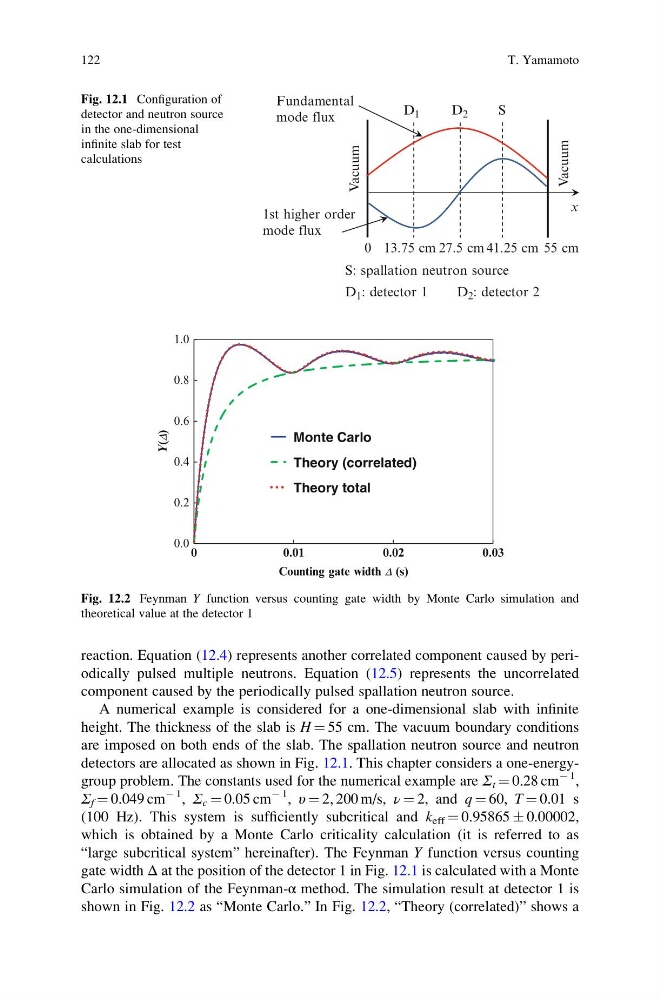
detectors are allocated as shown in Fig. 12.1. This chapter considers a one-energygroup problem. The constants used for the numerical example are Σ t ¼ 0.28 cm
À 1 ,
Σ f ¼ 0.049 cm
À 1 , Σ c ¼ 0.05 cm
À 1 , υ ¼ 2, 200 m/s, ν ¼ 2, and q ¼ 60, T ¼ 0.01 s
(100 Hz). This system is sufficiently subcritical and k eff ¼ 0.95865 Æ 0.00002,
which is obtained by a Monte Carlo criticality calculation (it is referred to as
“large subcritical system” hereinafter). The Feynman Y function versus counting
gate width Δ at the position of the detector 1 in Fig. 12.1 is calculated with a Monte
Carlo simulation of the Feynman-α method. The simulation result at detector 1 is
shown in Fig. 12.2 as “Monte Carlo.” In Fig. 12.2, “Theory (correlated)” shows a
Vacuum
Vacuum
0
x
D 1
D 2
S
13.75 cm 27.5 cm 41.25 cm 55 cm
S: spallation neutron source
D 1 : detector 1
Fundamental
mode flux
1st higher order
mode flux
D 2 : detector 2
Fig. 12.1 Configuration of
detector and neutron source
in the one-dimensional
infinite slab for test
calculations
0.0
0.2
0.4
0.6
0.8
1.0
0
0.01
0.02
0.03
Counting gate width D (s)
Y(D)
Monte Carlo
Theory (correlated)
Theory total
Fig. 12.2 Feynman Y function versus counting gate width by Monte Carlo simulation and
theoretical value at the detector 1
122
T. Yamamoto
component caused by the periodically pulsed spallation neutron source.
A numerical example is considered for a one-dimensional slab with infinite
height. The thickness of the slab is H ¼ 55 cm. The vacuum boundary conditions
are imposed on both ends of the slab. The spallation neutron source and neutron
detectors are allocated as shown in Fig. 12.1. This chapter considers a one-energygroup problem. The constants used for the numerical example are Σ t ¼ 0.28 cm
À 1 ,
Σ f ¼ 0.049 cm
À 1 , Σ c ¼ 0.05 cm
À 1 , υ ¼ 2, 200 m/s, ν ¼ 2, and q ¼ 60, T ¼ 0.01 s
(100 Hz). This system is sufficiently subcritical and k eff ¼ 0.95865 Æ 0.00002,
which is obtained by a Monte Carlo criticality calculation (it is referred to as
“large subcritical system” hereinafter). The Feynman Y function versus counting
gate width Δ at the position of the detector 1 in Fig. 12.1 is calculated with a Monte
Carlo simulation of the Feynman-α method. The simulation result at detector 1 is
shown in Fig. 12.2 as “Monte Carlo.” In Fig. 12.2, “Theory (correlated)” shows a
Vacuum
Vacuum
0
x
D 1
D 2
S
13.75 cm 27.5 cm 41.25 cm 55 cm
S: spallation neutron source
D 1 : detector 1
Fundamental
mode flux
1st higher order
mode flux
D 2 : detector 2
Fig. 12.1 Configuration of
detector and neutron source
in the one-dimensional
infinite slab for test
calculations
0.0
0.2
0.4
0.6
0.8
1.0
0
0.01
0.02
0.03
Counting gate width D (s)
Y(D)
Monte Carlo
Theory (correlated)
Theory total
Fig. 12.2 Feynman Y function versus counting gate width by Monte Carlo simulation and
theoretical value at the detector 1
122
T. Yamamoto