

the years 2036–2065). Various exposure parameters are available when comparing
climatic conditions from the past to the future (see Chaps. 2 and 3). This framework
selected the two exposure parameters corresponding most with the two plant indicators which describe the ecological envelope of a habitat. The mean temperature
(
C) indicates the changes in air temperature for each period and therefore can
describe the indicator temperature. The climatic water balance (mm) combines
precipitation and evapotranspiration and for that reason is one of the best parameter
to explain the distribution of vegetation (Stephenson 1990). The climatic water
balance indicates the changes in the water storage in the soil and therefore can be
used to be compared with the indicator moisture.
The exposure values were calculated as annual ensembles (for more details see
Chaps. 2 and 3). These values represented the climatic conditions during the course
of the year for the past and projected future date periods from above. Instead of the
usage of the length of the vegetation period, the productive time was divided into
three time segments, which are further referred to as 1/3, 2/3 and 3/3 of the
vegetation period. The non-productive time segment is referred as dormant period.
The exposure values therefore were calculated separately for each period during the
course of the year. First, the difference in the exposure values between the past and
future date period was obtained to get the amount of change from the past to the
future. This led to difference values ranging around zero (e.g. see Fig. 8.7 with
temperature range between 6 and À6
C). In a second step, the values were scaled
by dividing them by the root mean square. Now, the values of the different exposure
parameters (e.g.
C or mm) showed the same range around zero, which means that
all values at least range between 1 and À1. Finally, the scaled values were
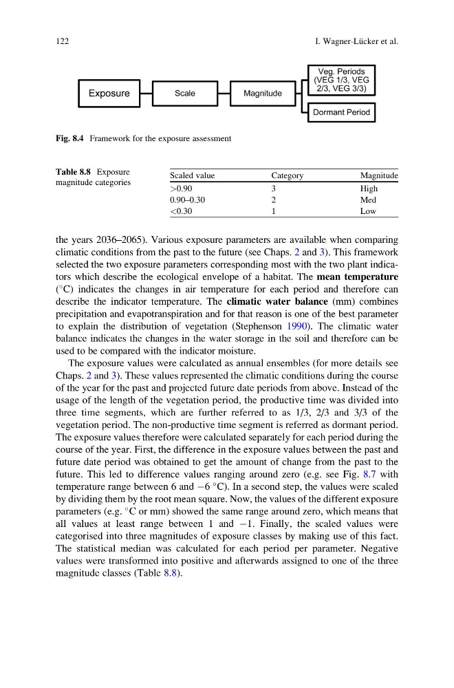
categorised into three magnitudes of exposure classes by making use of this fact.
The statistical median was calculated for each period per parameter. Negative
values were transformed into positive and afterwards assigned to one of the three
magnitude classes (Table 8.8).
Fig. 8.4 Framework for the exposure assessment
Table 8.8 Exposure
magnitude categories
Scaled value
Category
Magnitude
>0.90
3
High
0.90–0.30
2
Med
<0.30
1
Low
122
I. Wagner-Lu ¨cker et al.
climatic conditions from the past to the future (see Chaps. 2 and 3). This framework
selected the two exposure parameters corresponding most with the two plant indicators which describe the ecological envelope of a habitat. The mean temperature
(
C) indicates the changes in air temperature for each period and therefore can
describe the indicator temperature. The climatic water balance (mm) combines
precipitation and evapotranspiration and for that reason is one of the best parameter
to explain the distribution of vegetation (Stephenson 1990). The climatic water
balance indicates the changes in the water storage in the soil and therefore can be
used to be compared with the indicator moisture.
The exposure values were calculated as annual ensembles (for more details see
Chaps. 2 and 3). These values represented the climatic conditions during the course
of the year for the past and projected future date periods from above. Instead of the
usage of the length of the vegetation period, the productive time was divided into
three time segments, which are further referred to as 1/3, 2/3 and 3/3 of the
vegetation period. The non-productive time segment is referred as dormant period.
The exposure values therefore were calculated separately for each period during the
course of the year. First, the difference in the exposure values between the past and
future date period was obtained to get the amount of change from the past to the
future. This led to difference values ranging around zero (e.g. see Fig. 8.7 with
temperature range between 6 and À6
C). In a second step, the values were scaled
by dividing them by the root mean square. Now, the values of the different exposure
parameters (e.g.
C or mm) showed the same range around zero, which means that
all values at least range between 1 and À1. Finally, the scaled values were
categorised into three magnitudes of exposure classes by making use of this fact.
The statistical median was calculated for each period per parameter. Negative
values were transformed into positive and afterwards assigned to one of the three
magnitude classes (Table 8.8).
Fig. 8.4 Framework for the exposure assessment
Table 8.8 Exposure
magnitude categories
Scaled value
Category
Magnitude
>0.90
3
High
0.90–0.30
2
Med
<0.30
1
Low
122
I. Wagner-Lu ¨cker et al.